Verify the optimality condition for an optimal design (A-, c- or D-optimality)

Usage

plot_dispersion(
  u,
  design,
  tt,
  FUN,
  theta,
  criterion = "D",
  cVec = rep(0, length(theta))
)

Arguments

u: The discretized design points
design: The optimal design containing the design points and the associated weights
tt: The level of skewness
FUN: The function to calculate the derivative of the given model
theta: The parameter value of the model
criterion: The optimality criterion: one of "A", "c", or "D"
cVec: c vector used to determine the combination of the parameters. This is only used in c-optimality

Value

A plot verifying the general equivalence condition for the specified optimal design

Details

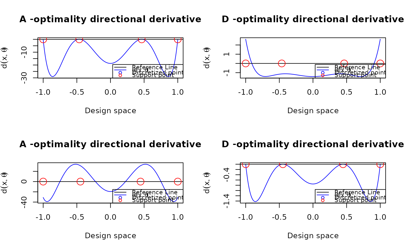
This function visualizes the directional derivative under A-, c-, or D-optimality using the general equivalence theorem. For an optimal design, the directional derivative should not exceed the reference threshold

Examples

poly3 <- function(xi, theta){
  matrix(c(1, xi, xi^2, xi^3), ncol = 1)
}
design_A <- data.frame(location = c(-1, -0.464, 0.464, 1),
                       weight = c(0.151, 0.349, 0.349, 0.151))
design_D = data.frame(location = c(-1, -0.447, 0.447, 1),
                      weight = rep(0.25, 4))
u <- seq(-1, 1, length.out = 201)
par(mfrow = c(2,2))
plot_dispersion(u, design_A, tt = 0, FUN = poly3, theta = rep(0, 4), criterion = "A")
plot_dispersion(u, design_A, tt = 0, FUN = poly3, theta = rep(0, 4), criterion = "D")

plot_dispersion(u, design_D, tt = 0, FUN = poly3, theta = rep(0, 4), criterion = "A")
plot_dispersion(u, design_D, tt = 0, FUN = poly3, theta = rep(0, 4), criterion = "D")