SLSEdesign

Optimal Design under Second-order Least Squares Estimator

Chi-Kuang Yeh and Julie Zhou
University of Waterloo and University of Victoria

2025-06-04

Installation

# required dependencies
require(SLSEdesign)
#> Loading required package: SLSEdesign
require(CVXR)
#> Loading required package: CVXR
#> 
#> Attaching package: 'CVXR'
#> The following object is masked from 'package:stats':
#> 
#>     power

Specify the input for the program

1. N: Number of design points

2. S: The design space

3. tt: The level of skewness

4. $\theta$: The parameter vector

5. FUN: The function for calculating the derivatives of the given model

N <- 21
S <- c(-1, 1)
tt <- 0
theta <- rep(1, 4)

poly3 <- function(xi,theta){
    matrix(c(1, xi, xi^2, xi^3), ncol = 1)
}

u <- seq(from = S[1], to = S[2], length.out = N)

res <- Aopt(N = N, u = u, tt = tt, FUN = poly3, 
            theta = theta)

Manage the outputs

Showing the optimal design and the support points

res$design
#>    location  weight
#> 1      -1.0 0.17905
#> 2      -0.9 0.00159
#> 3      -0.8 0.00310
#> 4      -0.7 0.00378
#> 5      -0.6 0.00346
#> 6      -0.5 0.00226
#> 8      -0.3 0.30676
#> 14      0.3 0.30676
#> 16      0.5 0.00226
#> 17      0.6 0.00346
#> 18      0.7 0.00378
#> 19      0.8 0.00310
#> 20      0.9 0.00159
#> 21      1.0 0.17905

Or we can plot them

plot_weight(res$design)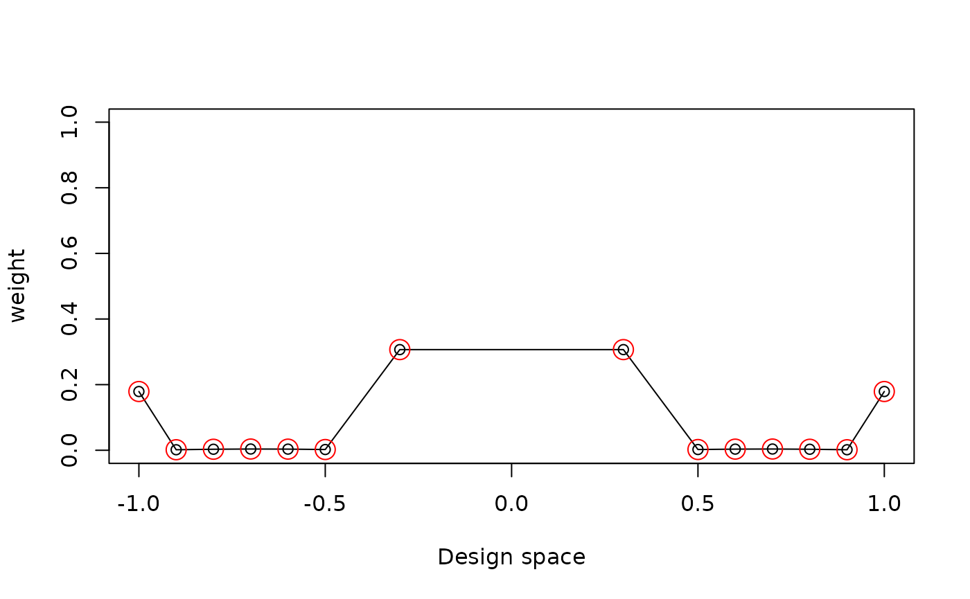

Plot the directional derivative to use the equivalence theorem for 3rd order polynomial models

D-optimal design

poly3 <- function(xi,theta){
    matrix(c(1, xi, xi^2, xi^3), ncol = 1)
}
design <- data.frame(location = c(-1, -0.447, 0.447, 1),
 weight = rep(0.25, 4))
u = seq(-1, 1, length.out = 201)
plot_dispersion(u, design, tt = 0, FUN = poly3,
  theta = rep(0, 4), criterion = "D")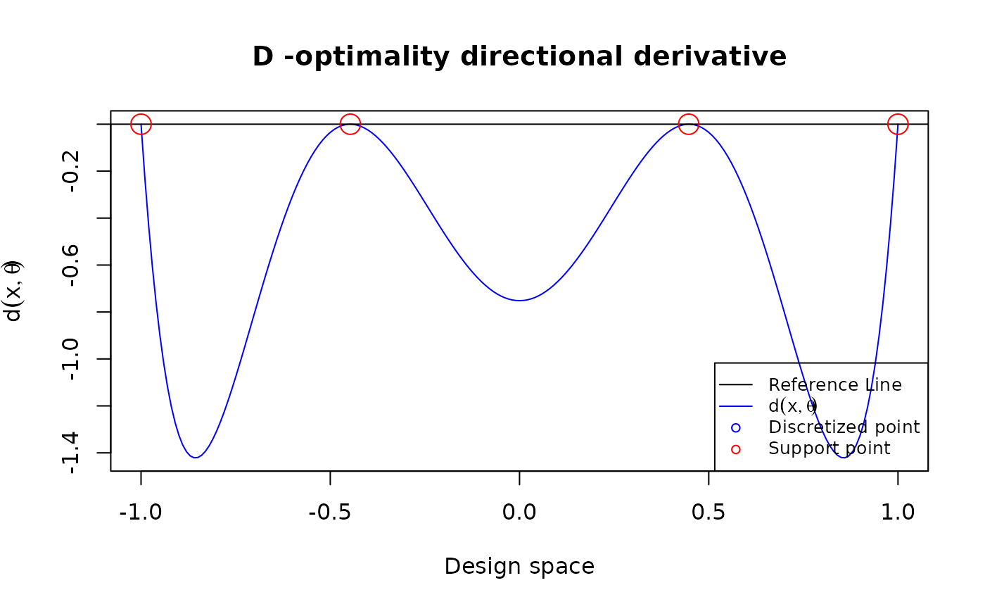

A-optimal design

poly3 <- function(xi, theta){
  matrix(c(1, xi, xi^2, xi^3), ncol = 1)
}
design <- data.frame(location = c(-1, -0.464, 0.464, 1),
                    weight = c(0.151, 0.349, 0.349, 0.151))
u = seq(-1, 1, length.out = 201)
plot_dispersion(u, design, tt = 0, FUN = poly3, theta = rep(0,4), criterion = "A")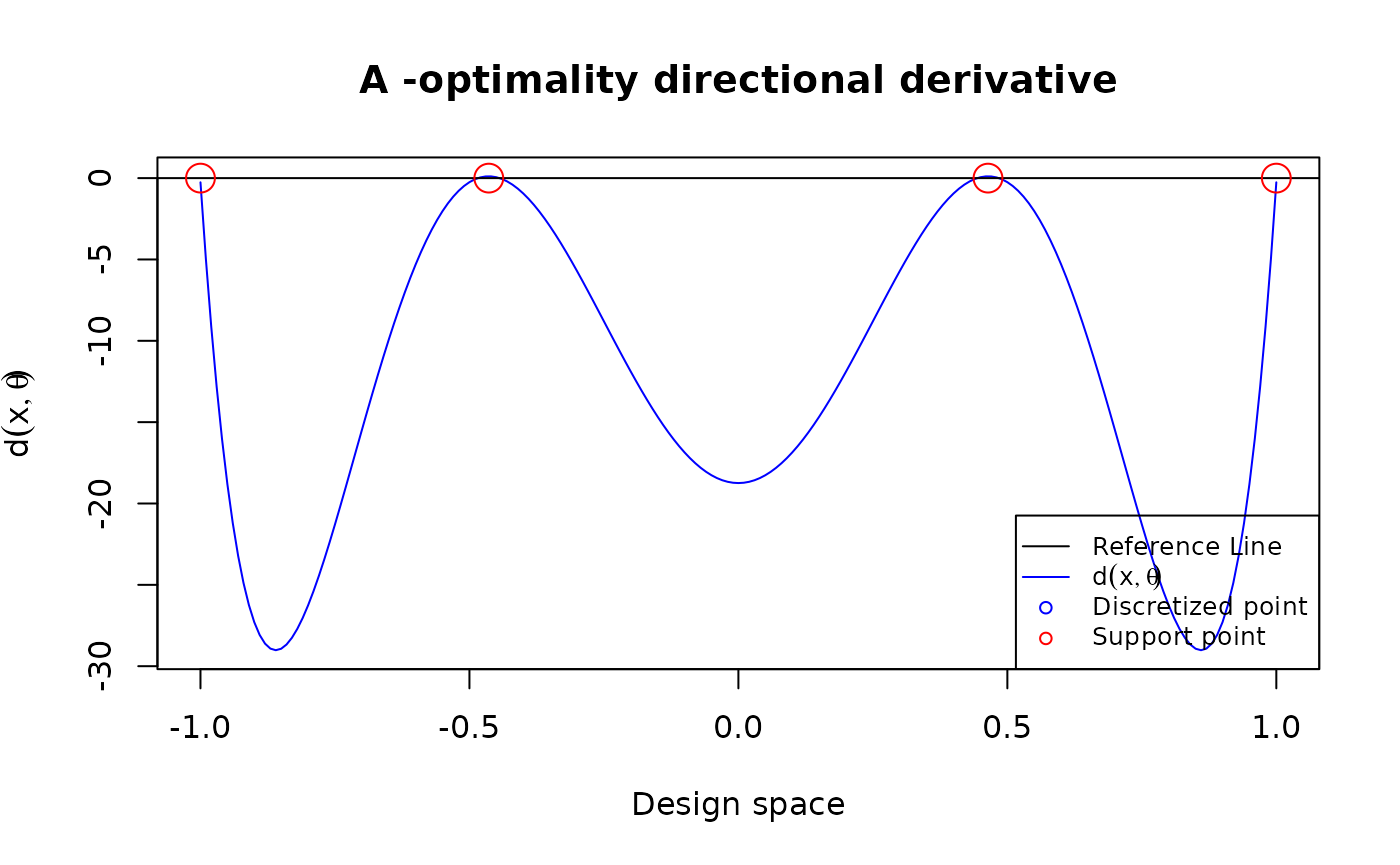

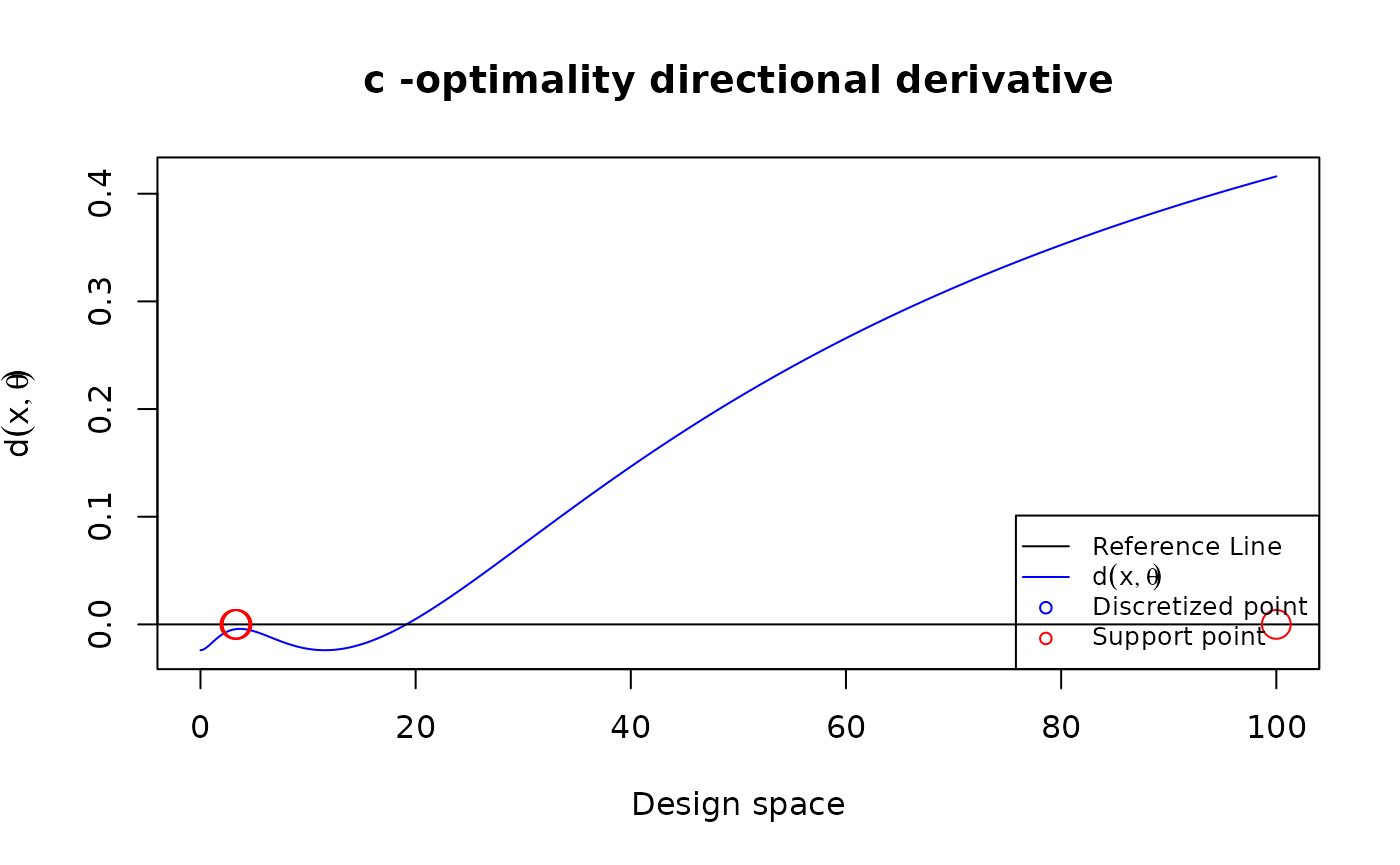
Plot the directional derivative to use the equivalence theorem for peleg model under c-optimality

my_peleg <- function(xi, theta) {
  deno <- (theta[1] + theta[2]*xi)
  matrix(c(-xi/deno^2, -xi^2/deno^2), ncol = 1)
}
Npt <- 1001
my_u <- seq(0, 100, length.out = Npt)
my_theta <- c(0.5, 0.05)
my_cVec <- c(1, 1)
my_design <- copt(
  N = Npt, u = my_u,
  tt = 0, FUN = my_peleg, theta = my_theta, num_iter = 50000,
  cVec = my_cVec
)

plot_dispersion(my_u, my_design$design, tt = 0, FUN = my_peleg, theta = my_theta, criterion = "c", cVec = my_cVec)