2  Week 1 — Introduction to Bayesian Thinking

---

2.1 Lecture 1: Motivation and Philosophy of the Bayesian Approach

2.1.1 1.1 Probability as Belief

• In the frequentist view, probability describes long-run frequencies of repeated events.
  
• In the Bayesian view, probability represents degrees of belief about uncertain quantities.
  This interpretation allows us to express uncertainty about parameters, models, and hypotheses.

2.1.2 1.2 Why Bayesian?

1. Unified logic of inference:
   All uncertainty (parameters, predictions, models) is treated probabilistically.
   
2. Incorporation of prior knowledge:
   Prior distributions let analysts integrate existing evidence or expert opinion.
   
3. Flexibility:
   The Bayesian framework handles hierarchical, missing-data, and complex models naturally.
   
4. Decision-theoretic foundation:
   Bayesian inference directly supports optimal decisions under uncertainty.
   
5. Computational advances:
   MCMC and modern probabilistic programming (e.g., Stan, PyMC, JAGS) make Bayesian analysis practical.

2.1.3 1.3 When to Use the Bayesian Approach

• Small-sample or sparse data problems where prior knowledge helps stabilize inference.
  
• Situations with sequential data collection or adaptive designs.
  
• Contexts demanding direct probability statements about parameters or hypotheses.
  
• Decision-making scenarios that require explicit uncertainty quantification.

2.1.4 1.4 Illustrative Example

Suppose a factory tests 10 light bulbs and finds 8 working.
- A frequentist estimates the proportion as 0.8 with a confidence interval.
- A Bayesian treats the true proportion \(\theta\) as random and updates beliefs via \(p(\theta \mid y) \propto p(y \mid \theta), p(\theta)\). The result: an explicit posterior distribution over \(\theta\), not a single point estimate.

---

2.2 Lecture 2: Bayes’ Theorem and the Building Blocks of Inference

2.2.1 2.1 Bayes’ Theorem

For parameters \(\theta\) and observed data \(y\):

\[ p(\theta \mid y) = \frac{p(y \mid \theta)\, p(\theta)}{p(y)} = \frac{p(y \mid \theta)\, p(\theta)}{\int p(y \mid \theta)\, p(\theta)\, d\theta}. \]

Where: - \(p(\theta)\): Prior — expresses beliefs before seeing data.
- \(p(y \mid \theta)\): Likelihood — the data-generating model.
- \(p(\theta \mid y)\): Posterior — updated belief after seeing data.
- \(p(y)\): Marginal likelihood / evidence — normalizing constant.

2.2.2 2.2 The Three Key Components

Component	Description	Example
Prior	Encodes information about \(\theta\) before data	\(\text{Beta}(2,~2)\) for coin bias
Likelihood	Probability model for data given \(\theta\)	\(\text{Binomial}(n=10,~\theta)\)
Posterior	Updated distribution combining both	\(\text{Beta}(2+y,~2+n-y)\)

2.2.3 2.3 Interpretation

• Posterior mean: expected value of \(\theta\) after observing data.
• Posterior credible interval: range where \(\theta\) lies with high probability (e.g., 95%).
• Posterior predictive distribution: used to predict future data.

2.2.4 2.4 Key Insight

The likelihood updates the prior in light of data — the posterior is the result of this update.

---

2.3 Lecture 3: Simple Analytical Examples of Bayesian Updating

2.3.1 3.1 Beta–Binomial Model (Coin-Flip Example)

Setup:
We flip a coin \(n\) times and observe \(y\) heads. Let \(\theta\) be the true probability of heads.

\[ y \mid \theta \sim \text{Binomial}(n, \theta), \quad \theta \sim \text{Beta}(\alpha_0, \beta_0). \]

Posterior: \[ \theta \mid y \sim \text{Beta}(\alpha_0 + y, \beta_0 + n - y). \]

Posterior mean: \[ E[\theta \mid y] = \frac{\alpha_0 + y}{\alpha_0 + \beta_0 + n}. \]

Interpretation:

• The prior acts as pseudo-data: \(\alpha_0 - 1\) prior successes and \(\beta_0 - 1\) prior failures.

• As \(n\) grows large, the data dominate the posterior.

Visualization:

Plot prior, likelihood, and posterior to show how the distribution tightens around the true value.

---

2.3.2 3.2 Normal–Normal Model (Inference on a Mean)

Setup:

Data \(y_1, \dots, y_n\) are i.i.d. \(\mathcal{N}(\mu, \sigma^2)\), with known variance \(\sigma^2\). We place a prior \(\mu \sim \mathcal{N}(\mu_0,~\tau_0^2)\).

Posterior:

\[ \mu \mid y \sim \mathcal{N}(\mu_1, \tau_1^2), \] where \[ \tau_1^2 = \left( \frac{1}{\tau_0^2} + \frac{n}{\sigma^2} \right)^{-1}, \quad \mu_1 = \tau_1^2 \left( \frac{\mu_0}{\tau_0^2} + \frac{n \bar{y}}{\sigma^2} \right). \]

Interpretation: The posterior mean is a weighted average of the prior mean and sample mean: \[ \mu_1 = w \mu_0 + (1-w)\bar{y}, \quad w = \frac{\sigma^2}{\sigma^2 + n\tau_0^2}. \]

When \(\tau_0^2\) is large (weak prior), \(\mu_1 \approx \bar{y}\). When data are scarce, the posterior leans more on the prior.

---

2.3.3 3.3 Posterior Predictive Distribution

For a future observation \[\tilde{y}:~p(\tilde{y} \mid y) = \int p(\tilde{y} \mid \theta), p(\theta \mid y), d\theta. \] Example (Beta–Binomial): \[ p(\tilde{y} = 1 \mid y) = E[\theta \mid y] = \frac{\alpha_0 + y}{\alpha_0 + \beta_0 + n}. \]

This predictive probability reflects both uncertainty in \(\theta\) and random variation in new data.

---

2.3.4 3.4 Discussion and Concept Reinforcement

• Priors influence the posterior most when data are limited.
• With sufficient data, Bayesian results converge to frequentist ones (Bernstein–von Mises theorem).
• Credible intervals directly express probability statements about parameters.
• Model assumptions (e.g., conjugacy, independence) simplify computation but can be relaxed using MCMC.

---

2.3.5 3.5 Practical Example (R Demonstration)

# Posterior update for a Binomial model
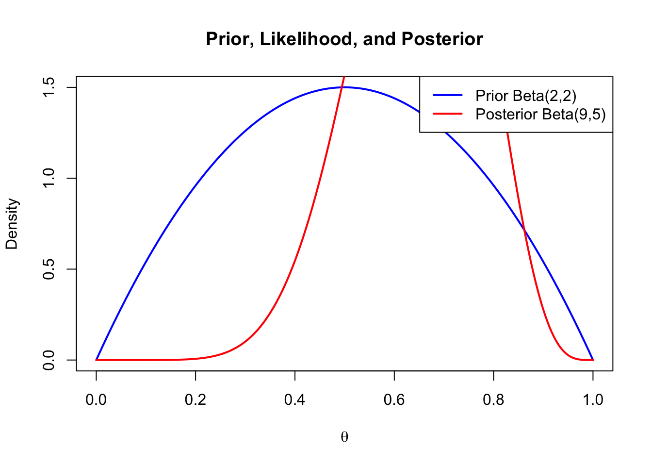
alpha0 <- 2; beta0 <- 2  # prior
n <- 10; y <- 7          # data
alpha1 <- alpha0 + y; beta1 <- beta0 + n - y

theta <- seq(0, 1, length.out = 500)
plot(theta, dbeta(theta, alpha0, beta0), type="l", lwd=2, col="blue",
     ylab="Density", xlab=expression(theta),
     main="Prior, Likelihood, and Posterior")
lines(theta, dbeta(theta, alpha1, beta1), col="red", lwd=2)
legend("topright",
       legend=c("Prior Beta(2,2)", "Posterior Beta(9,5)"),
       col=c("blue", "red"), lwd=2)