One of the fundamental tools required in computational statistics is the ability to simulate random variables (rvs) from specified probability distributions.
3.1 Overview
In the simplest case, to simulate drawing an observation at random from a finite population, a method of generating rvs from the discrete uniform distribution is required. Therefore, a suitable generator of uniform pseudo-random numbers is essential.
Methods for generating random variates from other probability distributions all depend on the uniform random number generator (RNG).
In the Appendices, we have seen that how to use the built-in R functions to generate RVs from some common distributions, such as runif(), rnorm(), rbinom(), etc. In this Section, we will go over some of the common methods to generate RVs from a costume distributions.
Example Theorem
If we already have a finite population of size \(N\) with values \(x_1, x_2, \ldots, x_N\) in hand, we can sample from this population with and without replacement.
set.seed(777)sample(c(0,1), size =10, replace =TRUE) # with replacement
 [1] "H" "N" "J" "Y" "B" "U" "F" "P" "Z" "V" "W" "I" "L" "A" "G" "Q" "X" "D" "M"
[20] "R" "C" "T" "O" "K" "E" "S"
Table 3.1: Common probability distributions and their corresponding R functions for cumulative distribution function (CDF) and random number generation (borrowed from Table 3.1 in reference [2]).
Distribution
cdf
Generator
Parameters
beta
pbeta
rbeta
shape1, shape2
binomial
pbinom
rbinom
size, prob
chi-squared
pchisq
rchisq
df
exponential
pexp
rexp
rate
F
pf
rf
df1, df2
gamma
pgamma
rgamma
shape, rate or scale
geometric
pgeom
rgeom
prob
lognormal
plnorm
rlnorm
meanlog, sdlog
negative binomial
pnbinom
rnbinom
size, prob
normal
pnorm
rnorm
mean, sd
Poisson
ppois
rpois
lambda
Student’s t
pt
rt
df
uniform
punif
runif
min, max
3.2 Inverse Transformation Method
The first method to simulate rvs is the inverse transformation method (ITM).
If \(X\sim F_X\) is a continuous rv, then the rv \(U = F_X(x) \sim \operatorname{Unif}(0,1)\).
ITM of generating rvs applies the probability integral transformation. Define the inverse transformation \[ F^{−1}_X(u) = \inf\{x : F_X(x) = u\},\quad 0 < u < 1.\] Then, if \(U \sim \operatorname{Unif}(0,1)\), the rv \(X = F^{−1}_X(U)\) has the distribution \(F_X\). This can be shown as, for all \(x \in \mathbb{R}\)
\[
\begin{aligned}
P\left(F_X^{-1}(U) \leq x\right) & =P\left(\inf \left\{t: F_X(t)=U\right\} \leq x\right) \\
& =P\left(U \leq F_X(x)\right) \\
& =F_U\left(F_X(x)\right)=F_X(x),
\end{aligned}
\] Hence, \(F_X^{-1}(U)\) and \(X\) have the same distribution. So, in order to generate rv \(X\), we can simulate \(U\sim \operatorname{Unif}(0,1)\) first, then apply the inverse \(F_X^{-1}(u)\).
NoteProcedure with inverse transformation method
Given a distribution function \(F_X(\cdot)\), we can simulate/generate a rv \(X\) using the ITM in three steps:
Derive the inverse function \(F_X^{-1}(u)\).
Write a (R) command or function to compute \(F_X^{-1}(u)\).
For each random variate required:
Generate a random \(u\sim \operatorname{Unif}(0,1)\).
Obtain \(x = F_X^{-1}(u)\).
3.2.1 Continuous case
When the distribution function \(F_X(\cdot)\) is continuous, the ITM is straightforward to implement.
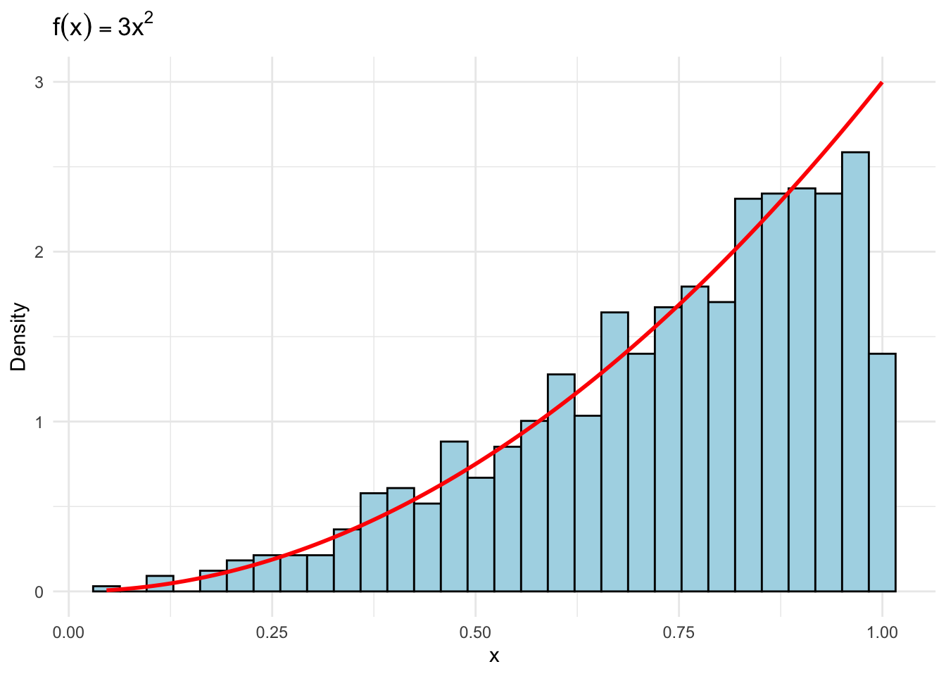
Suppose we want to use the ITM to simulate \(N=1000\) rvs from the density \(f_X(x)=3x^2,\quad x\in(0,1)\).
The cdf is \(F_X(x)=x^3\), so the inverse function is \(F_X^{-1}(u)=u^{1/3}\).
Simulate \(N=1000\) rvs from \(u\sim\operatorname{Unif}(0,1)\) and apply the inverse function to obtain the 1000 \(x\) values.
set.seed(777)N <-1000uVec <-runif(N)xVec <- uVec^(1/3)df <-data.frame(x = xVec)# Density histogram with theoretical density overlayggplot(df, aes(x)) +geom_histogram(aes(y = ..density..), bins =30,fill ="lightblue", color ="black") +stat_function(fun =function(x) 3*x^2,color ="red", size =1) +labs(title =expression(f(x) ==3*x^2),y ="Density", x ="x") +theme_minimal()
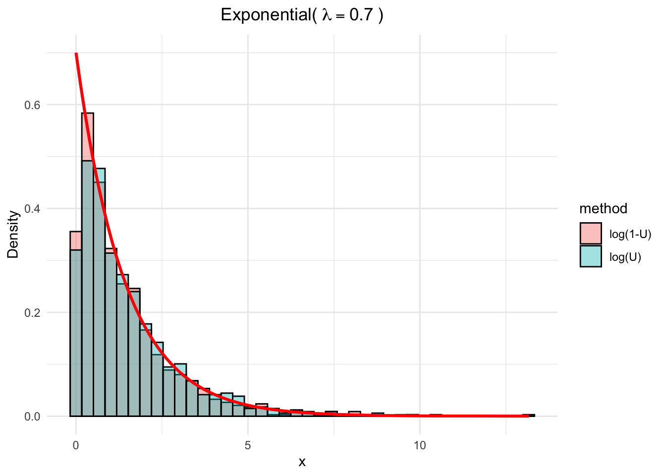
Suppose \(X\sim \exp(\lambda)\) where \(\lambda\) is the rate parameter. Then \(F_X(x) = 1 - e^{-\lambda x}\), so the inverse function is \(F_X^{-1}(u) = -\frac{1}{\lambda}\log(1-u)\). The other fact, is the \(U\) and \(1-U\) have the same distribution, so we can use either of them, i.e., \(x= -\frac{1}{\lambda}\log(u)\) or \(x= -\frac{1}{\lambda}\log(1-u)\).
set.seed(777)N <-1000lambda <-0.7uVec <-runif(N)xVec_1 <-- (1/lambda) *log(uVec)xVec_2 <-- (1/lambda) *log(1-uVec)# Put data into long format for ggplotdf <-data.frame(value =c(xVec_1, xVec_2),method =rep(c("log(U)", "log(1-U)"), each = N))# Theoretical density functionexp_density <-function(x) lambda *exp(-lambda * x)# Plotggplot(df, aes(x = value, fill = method)) +geom_histogram(aes(y = ..density..), bins =40,position ="identity", alpha =0.4, color ="black") +stat_function(fun = exp_density, color ="red", size =1) +labs(title =bquote("Exponential("~ lambda == .(lambda) ~")"),x ="x", y ="Density")
3.2.2 Discrete case
Although it is slightly more complicated than the continuous case, the ITM can also be applied to discrete distributions. Why?
First, in the discrete case, the cdf \(F_X(x)\) is NOT continuous, instead, a step function, so the inverse function \(F_X^{-1}(u)\) is not unique.
Here, if we order the random variable \[\cdots < x_{(i-1)} < x_{(i)} < x_{(i+1)}< cdots,\] then the inverse transformation is \(F_X^{-1}(u)=x_i\), where \(F_X(x_{(i-1)}) < u \leq F_X(x_{(i)})\).
Then the procedure is:
NoteProcedure with ITM for discrete case
Derive the cdf \(F_X(x)\) and tabulate the values of \(x_i\) and \(F_X(x_i)\).
Write a (R) command or function to compute \(F_X^{-1}(u)\).
For each random variate required:
Generate a random \(u\sim\operatorname{Unif}(0,1)\).
Find \(x_i\) such that \(F_X(x_{(i-1)}) < u \leq F_X(x_{(i)})\) and set \(x = x_i\).
In this example, \(F_X(0) = f_X(0) = 1 - p\) and \(F_X(1) = 1\).
Thus, \[
F_X^{-1}(u) =
\begin{cases}
1, & u > 0.6,\\
0, & u \leq 0.6.
\end{cases}
\]
The generator should therefore deliver the numerical value of the logical expression \(u > 0.6\).
set.seed(777)n <-1000p <-0.4u <-runif(n)x <-as.integer(u >0.6) # (u > 0.6) is a logical vector(m_x <-mean(x)); (v_x <-var(x))
[1] 0.381
[1] 0.2360751
Compare the sample statistics with the theoretical moments. The sample mean of a generated sample should be approximately \(p = 0.4\) and the sample variance should be approximately \(p(1 - p) = 0.24\), versus our simulated values 0.381 and 0.2360751.
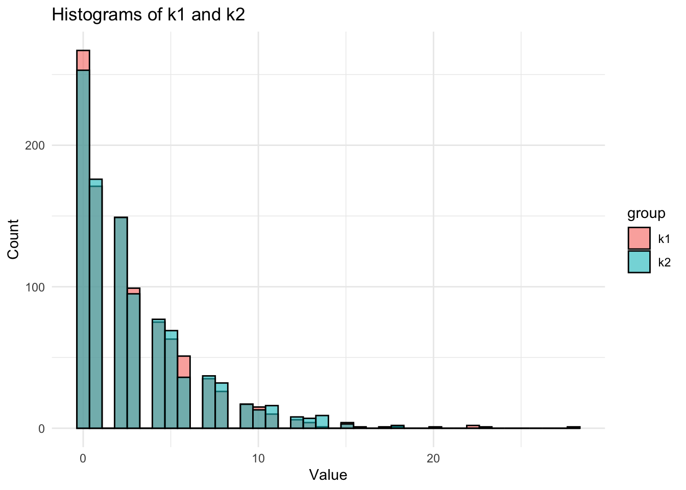
In this example, we will use ITM to simulate \(X\sim \operatorname{Geom}(1/4)\).
Let \(q:=1-p\). The pmf is \(f(x) = p q^x\), \(x = 0,1,2,\ldots\). At the points of discontinuity \(x = 0,1,2,\ldots\), the cdf is \[
F(x) = 1 - q^{x+1}.
\] For each sample element we need to generate a \(u\sim \operatorname{Unif}(0,1)\) and solve \[
1 - q^x < u \leq 1 - q^{x+1}.
\]
Which is equivalent to \(x < \frac{\log(1 - u)}{\log(q)} \leq x+1.\) The solution is \[
x + 1 = \left\lceil \frac{\log(1 - u)}{\log(q)} \right\rceil,
\] where \(\lceil \cdot \rceil\) denotes the ceiling function (and \(\lfloor \cdot \rfloor\) is the floor function). Hence, we have,
Note again that \(U\) and \(1 - U\) have the same distribution. Also, the probability that \(\log(1 - u)/\log(1 - p)\) equals an integer is zero. Thus, we can simplify it to
k2 <-floor(log(u) /log(1-p))df <-data.frame(value =c(k1, k2),group =rep(c("k1", "k2"), each =length(k1)))# Plot both histograms side by sideggplot(df, aes(x = value, fill = group)) +geom_histogram(alpha =0.6, position ="identity", bins =40, color ="black") +labs(title ="Histograms of k1 and k2", x ="Value", y ="Count") +theme_minimal()
The geometric distribution was particularly easy to simulate by the inverse transform method because it was easy to solve the inequality \(F(x-1) < u \leq F(x)\) rather than compare each \(u\) to all the possible values \(F(x)\).
The same method applied to the Poisson distribution is more complicated because we do not have an explicit formula for the value of \(x\) such that \[
F(x-1) < u \leq F(x).
\]
The R function generates random Poisson samples. The basic method to generate a Poisson (\(\lambda\)) variate is to generate and store the cdf via the recursive formula \[
f(x+1) = \frac{\lambda f(x)}{x+1},
\qquad
F(x+1) = F(x) + f(x+1).
\]
3.3 Acceptance-Rejection Method
In the previous section, we have seen that the ITM is straightforward to implement when the inverse cdf is available in closed form. However, for many distributions, the inverse cdf is not available in closed form or is difficult to compute. In those cases, we need to have other strategies!
The acceptance-rejection method (ARM) is a general method for generating rvs from a distribution with pdf \(f_X(x)\), when the inverse cdf is not available in closed form or is difficult to compute.
Suppose \(X\) and \(Y\) are rvs with pdfs/pmds \(f_X(x)\) and \(g_Y(y)\), respectively. Further we suppose there is a constant \(k\) such that \[
\frac{f_X(t)}{g_Y(t)} \leq k,
\] for all \(t\) such that \(f_X(t) > 0\).
Then we can simulate \(X\) using the following procedure:
Find a rv \(Y\) with density \(g_Y(\cdot)\) satisfying \(f_X(t)/g_Y(t) \le k,\) for all \(t\) such that \(f(t) > 0\).
For each rv, required:
Generate a random \(y\) from the distribution with density \(g_Y\).
Generate a random \(u\sim\operatorname{Unif}(0,1)\).
If \(u < f_X(y)/(k g_Y(y))\), accept \(y\) and set \(x = y\); o.w. reject \(y\) and jump back to (i)
Why it work?Note that in Step 2c, \[
P(\text{accept} \mid Y)
= P\!\left(U < \frac{f(Y)}{k g(Y)} \,\Big|\, Y\right)
= \frac{f_X(Y)}{k g_X(Y)}.
\]
The total probability of acceptance for any iteration is therefore \[
\sum_y P(\text{accept} \mid y) P(Y = y)
= \sum_y \frac{f(y)}{k g(y)} g(y)
= \frac{1}{k},
\] and the number of iterations until acceptance has the geometric distribution with mean \(k\). That means, in order to sample \(X\), in average, we need \(k\) iterations.
Note: The choice of \(Y\) and \(k\) is crucial for the efficiency of the ARM. A poor choice can lead to a large \(k\), resulting in many rejections and inefficiency. We want \(Y\) to be easy to simulate, and \(k\) to be as small as possible.
Does this have anything to do with \(X\)?
To see that the accepted sample has the same distribution as \(X\), apply Bayes’ Theorem. In the discrete case, for each \(\ell\) such that \(f(\ell) > 0\), \[
P(\ell \mid \text{accepted})
= \frac{P(\text{accepted} \mid \ell) g(\ell)}{P(\text{accepted})}
= \frac{\big[f(\ell)/(k g(\ell))\big] g(\ell)}{1/k}
= f(\ell).
\]
This example illustrates the acceptance–rejection method for the beta distribution.
Q: On average, how many random numbers must be simulated to generate \(N=1000\) samples from the \(\operatorname{Beta}(\alpha=2,\beta=2)\) distribution by ARM?
A: Depends on the upper bound \(k\) of \(f_X(t)/g_Y(t)\), which depends on the choice of the function \(g_Y(\cdot)\).
Recall that the \(\operatorname{Beta}(2,2)\) density is \[
f(t) = 6t(1-t), \quad 0 < t < 1.
\] Let \(g(\cdot)\) be the Uniform(0,1) density. Then \[
\frac{f(t)}{g(t)} = \frac{6t(1-t)}{(1)} = 6t(1-t) \leq k \quad \text{for all } 0 < t < 1.
\] It is easy to see that \(k = 6\). A random \(x\) from \(g(x)\) is accepted if \[
\frac{f(x)}{kg(x)} = \frac{6x(1-x)}{6(1)} = x(1-x) > u.
\]
On average, \(kN = 6\cdot 1000 =6000\) iterations (12000 random numbers as we need \(X\) and \(Y\)) will be required for \(N=1000\). In the following simulation, the counter \(\operatorname{iter}\) for iterations is not necessary, but included to record how many iterations were actually needed to generate the 1000 beta rvs.
set.seed(7777)N <-1000ell_accept <-0# counter for acceptediter <-0# iterationsy <-rep(0, N)while (ell_accept < N) { u <-runif(1) iter <- iter +1 x <-runif(1) # random variate from gif (x * (1-x) > u) {# we accept x ell_accept <- ell_accept +1 y[ell_accept] <- x }}iter
[1] 5972
In this simulation, 5972 iterations ( 1.1944^{4} random numbers) were required to generate the 1000 beta samples.
3.4 Using known probability distribution theory
Many types of transformations other than the probability inverse transformation can be applied to simulate random variables. Some examples are
1). If \(Z \sim N(0,1)\), then \(V = Z^2 \sim \chi^2(1)\).
2). If \(Z_1,\ldots,Z_n \sim N(0,1)\) are independent, then \[
U = \sum_{i=1}^n Z_i^2 \sim \chi^2(n).
\]
3). If \(U \sim \chi^2(m)\) and \(V \sim \chi^2(n)\) are independent, then \[
F = \frac{U/m}{V/n}
\] has the \(F\) distribution with \((m,n)\) degrees of freedom.
4). If \(Z \sim N(0,1)\) and \(V \sim \chi^2(n)\) are independent, then \[
T = \frac{Z}{\sqrt{V/n}}
\] has the Student \(t\) distribution with \(n\) degrees of freedom.
5). If \(U,V \sim \text{Unif}(0,1)\) are independent, then \[
Z_1 = \sqrt{-2 \log U}\, \cos(2\pi V),
\qquad
Z_2 = \sqrt{-2 \log U}\, \sin(2\pi V)
\] are independent standard normal variables.
6). If \(U \sim \text{Gamma}(r,\lambda)\) and \(V \sim \text{Gamma}(s,\lambda)\) are independent, then \[
X = \frac{U}{U+V}
\] has the \(\text{Beta}(r,s)\) distribution.
7). If \(U,V \sim \text{Unif}(0,1)\) are independent, then \[
X = \left\lfloor 1 + \frac{\log(V)}{\log\big(1 - (1-\theta)U\big)} \right\rfloor.
\] has logarithmic distribution with parameter \(\theta\).
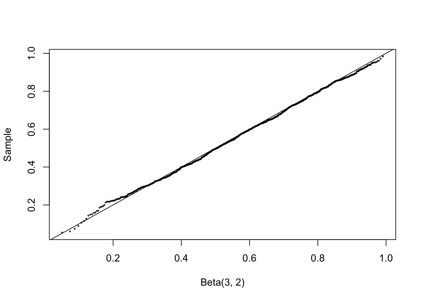
Using the distribution theory, we recall the relationship between beta and gamma distributions provides another beta generator.
If \(U \sim \mathrm{Gamma}(r,\lambda)\) and \(V \sim \mathrm{Gamma}(s,\lambda)\) are independent, then \[
X=\frac{U}{U+V}
\] has the \(\mathrm{Beta}(r,s)\) distribution. This transformation determines an algorithm for generating random \(\mathrm{Beta}(a,b)\) variates.
Generate a random \(u\) from \(\mathrm{Gamma}(a,1)\).
Generate a random \(v\) from \(\mathrm{Gamma}(b,1)\).
Obtain \(x=\dfrac{u}{u+v}\).
This method is applied below to generate a random \(\mathrm{Beta}(3,2)\) sample.
set.seed(777)n <-1000a <-3b <-2u <-rgamma(n, shape = a, rate =1)v <-rgamma(n, shape = b, rate =1)x <- u / (u + v)
The sample data can be compared with the Beta\((3,2)\) distribution using a quantile–quantile (QQ) plot. If the sampled distribution is Beta\((3,2)\), the QQ plot should be nearly linear.
Let \(X_1, X_2, \ldots, X_n \overset{iid}{\sim}F_X\). Then we may consider the sum of the random variables \(S_n:=\sum_{i=1}^n X_i\), with distribution \(F_{S_n}\), which can be referred as convoluton. We can simulate \(S_n\) by simulating \(X_1, X_2, \ldots, X_n\) and summing them up. There are several common convolutions we have seen so far
Sum of \(n\) independent i.i.d. chi-square with degreee of freedom (df) 1 is chi-square with df \(n\).
Sum of \(n\) independent i.i.d. exponential with rate \(\lambda\) is gamma with shape \(n\) and rate \(\lambda\).
Sum of \(n\) independent i.i.d. geometric with parametric \(p\) is negative binomial with size \(n\) and parameter \(p\).
In order to simulate \(\chi^2\) distribution with df k, we can simulate k independent standard normal rvs and sum their squares. Let’s simulate \(n\) independent \(S \sim \chi^2(5)\).
Fill an \(n \times k\) matrix with \(n k\) realization of the random variables that follow \(N(0,1)\).
Square each entry in the matrix (1).
Compute the row sums of the squared normals. Each row sum is one random observation from the \(\chi^2(k)\) distribution.
A mixture distribution is a probability distribution constructed as a weighted sum of other distributions. If \(X\) is a rv with a mixture distribution, then its pdf is given by \[
F_X(x) = \sum_{i=1}^k \alpha_i F_{X_i}(x),
\] where \(\alpha_i\ge 0\) and \(\sum_i \alpha_i=1\). We can just simply simulate each component\(X_i\) first, then multiply with their corresponding weights \(\alpha_i\).
Suppose \(X\) and \(Y\) is a mixture of two normal distributions, where \(X\sim N(\mu_1,\sigma_1^2)\) with probability \(\alpha\) and \(Y\sim N(\mu_2,\sigma_2^2)\) with probability \(1-\alpha\).
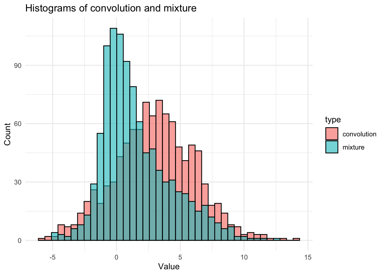
n <-1000x1 <-rnorm(n, 0, 1)x2 <-rnorm(n, 3, 3)s_convolution <- x1 + x2 #the convolutionu <-runif(n)k <-as.integer(u >0.5) #vector of 0’s and 1’s## pay attention to itm_mixture <- k * x1 + (1-k) * x2 #the mixturedf <-data.frame(value =c(s_convolution, m_mixture),type =rep(c("convolution", "mixture"), each = n))ggplot(df, aes(x = value, fill = type)) +geom_histogram(alpha =0.6, position ="identity", bins =40, color ="black") +labs(title ="Histograms of convolution and mixture", x ="Value", y ="Count") +theme_minimal()
NoteSimulate for mixture
Pay attention how a mixture is simulated. In particular, we first simulate a vector \(U\sim\operatorname{Unif}(0,1)\), then use it to select from which distribution/component we want to sample. It is not an (weighted) addition as in the convolution.
NoteDifference between convolution and mixture
Convolution is the sum of two independent rvs, while mixture is a weighted average of two rvs. Note: Mixture is non-normal! but the convolution is normal.
3.6 Simulate Multivaraite RVs
This section presents generators for the multivariate normal distribution, multivariate normal mixtures, the Wishart distribution, and the uniform distribution on the sphere in \(\mathbb{R}^d\).
3.6.1 Multivariate normal distribution
Recall that, from Definition 1 in Chapter 2, a \(d\)-dimensional random vector \(X\) is a multivariate normal distribution with mean vector \(\mu\) and covariance matrix \(\Sigma\), denoted by \(X \sim N_d(\mu, \Sigma)\), if every linear combination of its components has a univariate normal distribution. That is, for every nonzero vector \(a \in \mathbb{R}^d\), the rv \(a^T X\) has a univariate normal distribution.
To write this in an explicit form, we have, \(X = (X_1,\dots,X_N)\) follow a multivariate normal (MVN) distribution with mean vector \(\mu = (\mu_1,\dots,\mu_N)\) and covariance matrix \(\Sigma = (\sigma_{ij})\), if its joint density function is given by \[
f_X(x) = \frac{1}{(2\pi)^{p/2} |\Sigma|^{1/2}} \exp\left(-\frac{1}{2}(x - \mu)^T \Sigma^{-1} (x - \mu)\right), \quad x \in \mathbb{R}^p.
\]
More explicitly, we can write this as the \[\mu=(\mu_1,\dots,\mu_p) = \begin{pmatrix}\mu_1\\
\vdots\\
\mu_p\end{pmatrix}\in \mathbb{R}^p,\] and \[\Sigma=(\Sigma_{ij}) = (\mathbb{C}ov(X_i,X_j))= \left[\begin{array}{cccc}
\sigma_{11} & \sigma_{12} & \ldots & \sigma_{1 d} \\
\sigma_{21} & \sigma_{22} & \ldots & \sigma_{2 d} \\
\vdots & \vdots & & \vdots \\
\sigma_{d 1} & \sigma_{d 2} & \ldots & \sigma_{d d}
\end{array}\right] \in \mathbb{R}^{d\times d}.
\]
A random vector \(X\sim N_d(\mu,\Sigma)\) can be simulated by the following steps:
Simulate \(Z = (Z_1,\ldots,Z_d)^T\) where \(Z_i \overset{iid}{\sim}N(0,1)\).
Find a vector \(\mu\) and a matrix \(A\) and such that \(\Sigma = AA^T\). The decomposition can be Cholesky decomposition, eigendecomposition, or singular value decomposition, etc.
In practice, we do not do this one at a time, we want to simulate \(n\) sample in as few steps as possible. The following procedure is more efficient. Typically, one applies the transformation to a data matrix and transforms the entire sample. Suppose that \(Z = (Z_ij ) \in \mathbb{R}^{n\times d}\), where \(Z_{ij}\overset{iid}{\sim}N(0,1)\). Then the rows of Z are \(n\) random observations from the \(d\)-dimensional standard MVN distribution. The required transformation applied to the data matrix is \[X = ZQ + J \mu^\top,\] where \(Q^\top Q=\Sigma\), and \(J\) is a column vector of \(n\) ones. The rows of \(X\) are \(n\) random observations from the \(d\)-dimensional MVN distribution with mean vector \(\mu\) and covariance matrix \(\Sigma\).
Method for generating multivariate $n $ normal samples from the \(N_d(\mu,\Sigma)\) distribution.
Step 2. Compute the decomposition \(\Sigma = Q^\top Q\).
Step 3. Compute \(X = ZQ + J\mu^\top\), where \(J\) is a column vector of \(n\) ones.
Step 4. Return \(X\in \mathbb{R}^{ n\times d}\), in which each of the \(n\) rows of \(X\) is a random observation from the \(N_d(\mu,\Sigma)\) distribution.
3.6.1.1 A few things to be considered
Computation of \(J \mu^\top\)
Recall that \(J\) is a vector of 1’s (i.e., \(J=(1,\dots,1)\in\mathbb{R}^d\) and \(\mu^\top\) is the transpose of \(\mu\). So, \(J \mu^\top\) is a matrix with each row being \(\mu\). In R, we can use matrix(mu, n, d, byrow = TRUE) to create this matrix. Also, for any \(i\) and \(j\), \(\mu_i=\mu_j=c\), where c is a constant, then we can write it as \(c I_{n\times d}\), where \(I_{n\times d}\) is a matrix of 1’s with dimension \(n\times d\).
Z <-matrix(rnorm(n*d), nrow = n, ncol = d)X <- Z %*% Q +matrix(mu, n, d, byrow =TRUE)
Decomposition of \(\Sigma\)
There are many different ways to decompose \(\Sigma\). Recall that \(\Sigma\) is a symmetric positive definite matrix, so we can use Cholesky decomposition, eigendecomposition, or singular value decomposition (SVD). In R, we can use chol(), eigen(), or svd() functions to compute the decomposition.
Choleski decomposition: Choleski of a real symmetric positive-definite matrix is \(X = Q^\top Q\), where \(Q\) is an upper triangular matrix.
Spectral decomposition: The square root of the covariance is \(Σ^{1/2} = P^{1/2} \Lambda P^{−1}\), where \(\Lambda\) is the diagonal matrix with the eigenvalues of \(\Sigma\) along the diagonal and \(P\) is the matrix whose columns are the eigenvectors of \(\Sigma\) corresponding to the eigenvalues in \(\Lambda\). This method can also be called the eigen-decomposition method. In the eigen-decomposition we have \(P^{-1}= P^\top\) and therefore \(Σ^{1/2} = P \Lambda^{1/2}P^\top\) . The matrix \(Q = Σ^{1/2}\) is a factorization of \(\Sigma\) such that \(Q^\top Q = \Sigma\).
Singular Value Decomposition: The singular value decomposition (svd) generalizes the idea of eigenvectors to rectangular matrices. The svd of a matrix \(X\) is \(X = U DV^\top\) , where D is a vector containing the singular values of \(X\), \(U\) is a matrix whose columns contain the left singular vectors of \(X\), and \(V\) is a matrix whose columns contain the right singular vectors of \(X\). The matrix \(X\) in this case is the population covariance matrix \(\Sigma\), and \(UV\top = I\). The svd of a symmetric positive definite matrix \(\Sigma\) gives \(U = V = P\) and \(Σ^{1/2} = U D^{1/2}V^\top\) . Thus the svd method for this application is equivalent to the spectral decomposition method, but is less efficient because the svd method does not take advantage of the fact that the matrix \(\Sigma\) is square symmetric.
NotePerformance Comparison
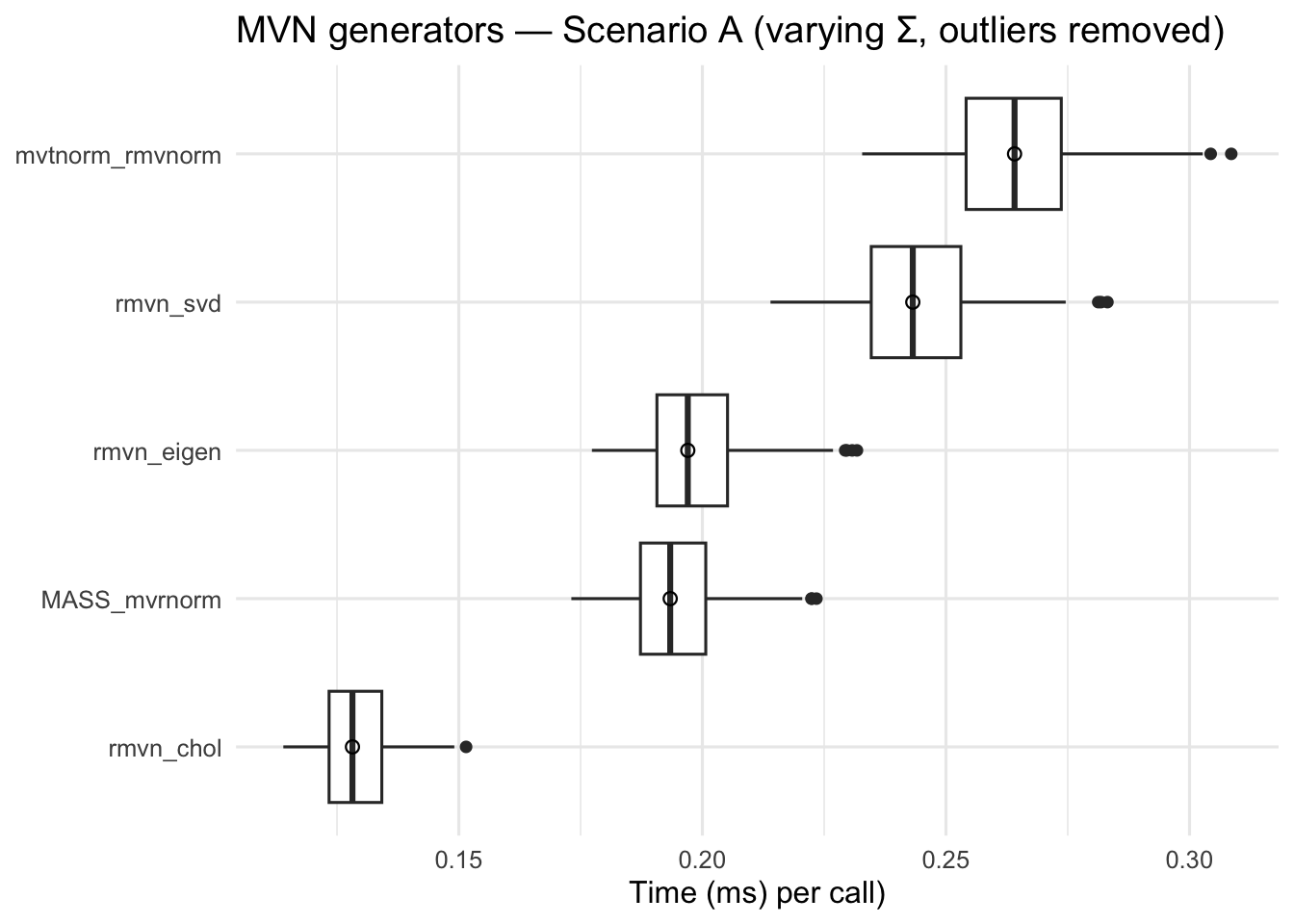
set.seed(777)n <-100# sample size per calld <-30# dimensionN <-1000# number of distinct Sigmas to cycle through in Scenario Areps_A <-200# microbenchmark repetitions for Scenario Areps_B <-500# microbenchmark repetitions for Scenario Bmu <-numeric(d)## ====== MVN generators ======rmvn_eigen <-function(n, mu, Sigma) { ev <-eigen(Sigma, symmetric =TRUE) A <- ev$vectors %*% (sqrt(pmax(ev$values, 0)) *t(ev$vectors)) Z <-matrix(rnorm(n *length(mu)), n)sweep(Z %*% A, 2, mu, `+`)}rmvn_svd <-function(n, mu, Sigma) { sv <-svd(Sigma) A <- sv$u %*% (sqrt(pmax(sv$d, 0)) *t(sv$v)) Z <-matrix(rnorm(n *length(mu)), n)sweep(Z %*% A, 2, mu, `+`)}rmvn_chol <-function(n, mu, Sigma) { R <-chol(Sigma) Z <-matrix(rnorm(n *length(mu)), n)sweep(Z %*% R, 2, mu, `+`)}## ====== Utilities ======rand_cov <-function(d) { A <-matrix(rnorm(d*d), d, d) S <-crossprod(A) / ddiag(S) <-diag(S) +1e-6 S}drop_outliers <-function(df) { df %>%group_by(expr) %>%mutate(q1 =quantile(time, 0.25),q3 =quantile(time, 0.75),iqr = q3 - q1,lower = q1 -1.5* iqr,upper = q3 +1.5* iqr ) %>%filter(time >= lower & time <= upper) %>%ungroup()}## Precompute N random SPD matrices (same pool for all methods)Sigma_list <-replicate(N, rand_cov(d), simplify =FALSE)## ====== Scenario A: varying Sigma each call (factorize every time) ======i <-0next_Sigma <-function() { i <<-if (i == N) 1else i +1; Sigma_list[[i]] }bench_A <-microbenchmark(rmvn_eigen =rmvn_eigen(n, mu, next_Sigma()),rmvn_svd =rmvn_svd(n, mu, next_Sigma()),rmvn_chol =rmvn_chol(n, mu, next_Sigma()),MASS_mvrnorm = MASS::mvrnorm(n, mu, next_Sigma()),mvtnorm_rmvnorm = mvtnorm::rmvnorm(n, mean = mu, sigma =next_Sigma()),times = reps_A)sum_A <-as.data.frame(bench_A) %>%group_by(expr) %>%summarize(median_ms =median(time)/1e6,iqr_ms =IQR(time)/1e6,.groups ="drop") %>%arrange(median_ms) %>%mutate(scenario ="A: varying Σ")print(sum_A)
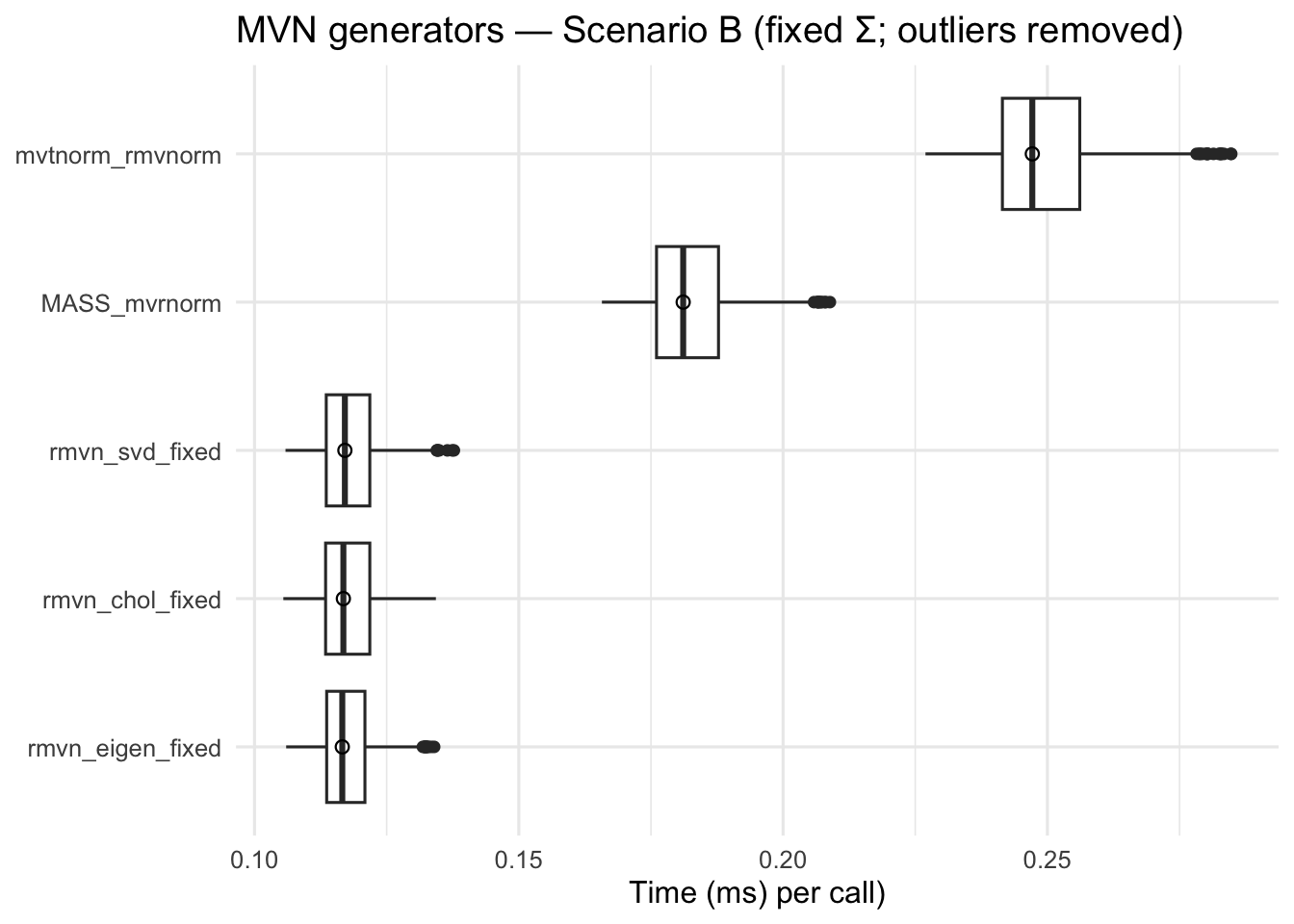
pB <-drop_outliers(as.data.frame(bench_B)) %>%mutate(ms = time/1e6) %>%ggplot(aes(x =reorder(expr, ms, FUN = median), y = ms)) +geom_boxplot() +stat_summary(fun = median, geom ="point", shape =21, size =2, stroke =0.6) +coord_flip() +labs(title ="MVN generators — Scenario B (fixed Σ; outliers removed)",x =NULL, y ="Time (ms) per call)") +theme_minimal(base_size =12)print(pB)
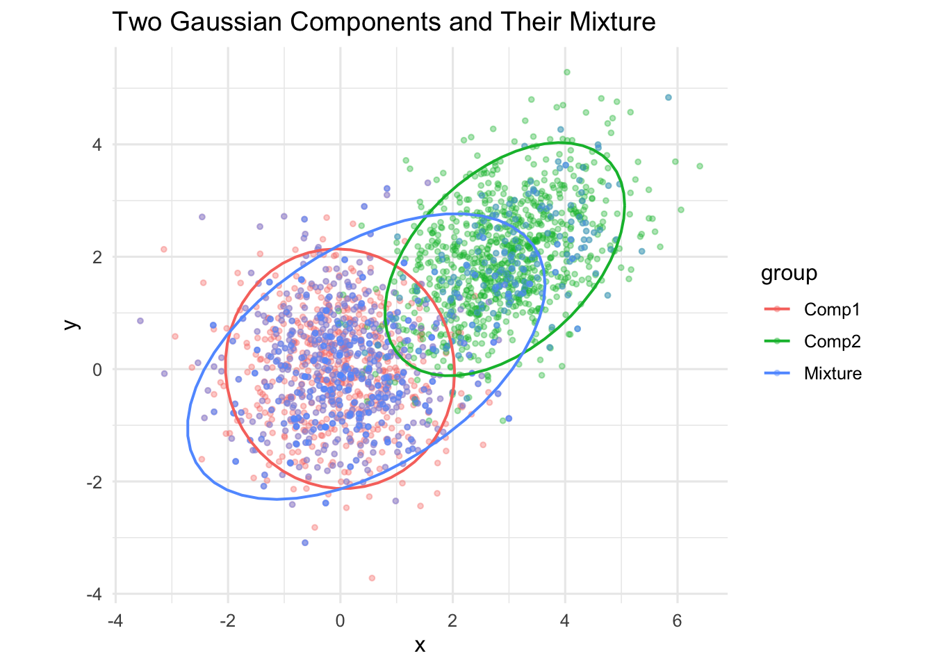
3.6.2 Mixture of Multivariate Normal
A mixture of multivariate normal distributions is a convex combination of multivariate normal distributions. That is, the density function of a mixture of \(k\) multivariate normal distributions is given by \[
\alpha N_p(\mu_1,\Sigma_1) + (1-\alpha) N_p(\mu_2,\Sigma_2), \quad 0 < \alpha < 1.
\] Similar to the univariate case, different choice of \(\alpha\) will lead to different degree of departure from the normal.
Given a \(\alpha\), to simulatecallout-note a random sample from \(\alpha N_d(\mu_1, \Sigma_1) + (1 − p) N_d(\mu_2, \Sigma_2)\)
There are two ways.
Way 1:
Generate \(U \sim unif(0,1) \in \mathbb{R}^n\).
(Component-wise) If \(U_i \le \alpha\), generate X from \(X_i\sim N_d(\mu_1, \Sigma_1)\), o.w. generate \(X_i from \sim N_d(\mu_2, \Sigma_2)\).
(Component-wise) If \(N_i = 1\) generate \(X\) from \(X_i \sim N_d(\mu_1, \Sigma_1)\), o.w. generate \(X\) from \(N_d(\mu_2, \Sigma_2)\).
set.seed(777)loc.mix.0<-function(n, alpha, mu1, mu2, Sigma) {# generate sample from BVN location mixture X <-matrix(0, n, 2)for (i in1:n) { k <-rbinom(1, size =1, prob = alpha)if (k) { X[i, ] <-mvrnorm(1, mu = mu1, Sigma) } else { X[i, ] <-mvrnorm(1, mu = mu2, Sigma) } }return(X)}
loc.mix <-function(n, alpha, mu1, mu2, Sigma) {# generate sample from BVN location mixture n1 <-rbinom(1, size = n, prob = alpha) n2 <- n - n1 x1 <-mvrnorm(n1, mu = mu1, Sigma) x2 <-mvrnorm(n2, mu = mu2, Sigma) X <-rbind(x1, x2) # combine the samplesreturn(X[sample(1:n), ]) # mix them}
NoteMixture of multivariate normal
One interesting example is when \(\alpha = 1 − 1/2 (1 − \sqrt{3}/3 )\approx .
0.7887\), provides an example of a skewed distribution with normal kurtosis (level of the peak).
set.seed(777)n <-1000comp1 <- MASS::mvrnorm(n, mu =c(0, 0), Sigma =diag(2))comp2 <- MASS::mvrnorm(n, mu =c(3, 2), Sigma =matrix(c(1, 0.5, 0.5, 1), 2))# Proper mixture membership per observationalpha <-1-1/2*(1-sqrt(3)/3 ) # P(Comp1)memb <-rbinom(n, 1, alpha) # 1 = Comp1, 0 = Comp2# Build the mixture matrix row-wise (avoid ifelse on matrices)mix <-matrix(NA_real_, nrow = n, ncol =2)id1 <- memb ==1id2 <-!id1mix[id1, ] <- comp1[sample(n, sum(id1), replace =TRUE), ]mix[id2, ] <- comp2[sample(n, sum(id2), replace =TRUE), ]# Tidy data frames with labelsdf1 <-data.frame(x = comp1[,1], y = comp1[,2], group ="Comp1")df2 <-data.frame(x = comp2[,1], y = comp2[,2], group ="Comp2")dfm <-data.frame(x = mix[,1], y = mix[,2], group ="Mixture")df_all <-rbind(df1, df2, dfm)# Option A: single panel, colored by groupp1 <-ggplot(df_all, aes(x, y, color = group)) +geom_point(alpha =0.35, size =1) +stat_ellipse(level =0.95, linewidth =0.7) +coord_equal() +theme_minimal(base_size =12) +labs(title ="Two Gaussian Components and Their Mixture")p1
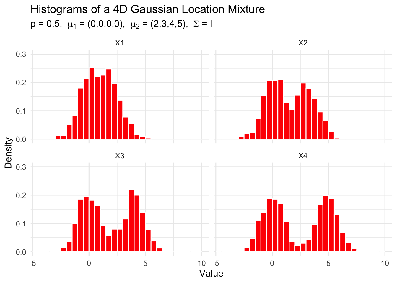
NoteHigher dimensional case
It is difficult to visualize data in \(R^d\), for \(d\ge 4\), so we display only the histograms of the marginal distributions. All of the one-dimensional marginal distributions are univariate normal location mixtures.
set.seed(777)library(MASS)library(ggplot2)library(tidyr)# ---- generate x exactly like your call ----x <-loc.mix(1000, .5, rep(0, 4), 2:5, Sigma =diag(4))colnames(x) <-paste0("X", 1:4)# ---- ggplot histograms ----r <-range(x) *1.2# global x-limits like your base R codedf_long <-as.data.frame(x) |>pivot_longer(everything(), names_to ="Variable", values_to ="Value")ggplot(df_long, aes(x = Value)) +geom_histogram(aes(y = ..density..),breaks =seq(-5, 10, 0.5),fill ="red", color ="white") +facet_wrap(~ Variable, ncol =2) +coord_cartesian(xlim = r, ylim =c(0, 0.3)) +theme_minimal(base_size =12) +labs(title ="Histograms of a 4D Gaussian Location Mixture",subtitle =expression(paste("p = 0.5, ", mu[1], " = (0,0,0,0), ", mu[2], " = (2,3,4,5), ", Sigma, " = I")),x ="Value", y ="Density" )
Warning: The dot-dot notation (`..density..`) was deprecated in ggplot2 3.4.0.
ℹ Please use `after_stat(density)` instead.
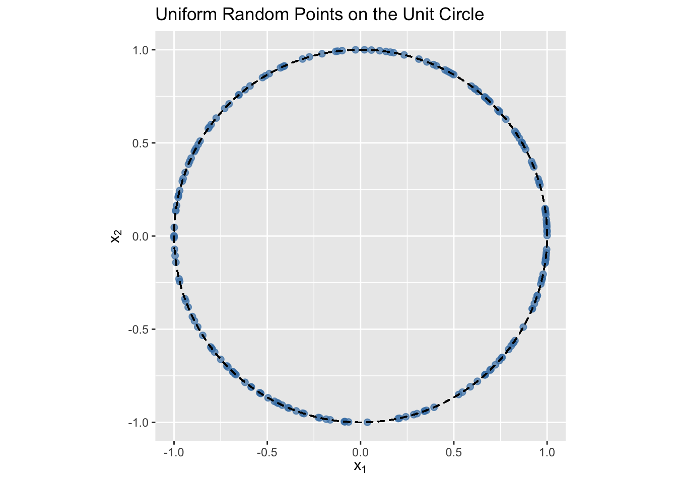
3.6.3 Uniform Distribution on a Sphere
The uniform distribution on the surface of a \(d\)-sphere in \(\mathbb{R}^d\) is the distribution that assigns equal probability to equal areas on the surface of the sphere.
The d-sphere is the set of all points \(x \in \mathbb{R}^d\) such that \(\| x \| = \sqrt{x^\top x} = 1\). Random vectors uniformly distributed on the \(d\)-sphere have equally likely directions. A method of generating this distribution uses a property of the
multivariate normal distribution (see [97, 160]). If X1, . . . , Xd are iid N (0, 1), then U = (U1, . . . , Ud) is uniformly distributed on the unit sphere in Rd, where
\[
U_j=\frac{X_j}{\left(X_1^2+\cdots+X_d^2\right)^{1 / 2}}, \quad j=1, \ldots, d \tag{*}
\]
Algorithm to generate uniform variates on the \(d\)-Sphere
For each variate \(u_i,~ i = 1,\dots , n\) repeat
Generate a random sample \(x_{i_1}, \dots , x_{i_d}\) from \(N (0, 1)\).
To implement these steps efficiently in R for a sample size n,
Generate nd univariate normals in \(n \times d\) matrix \(M\). The \(i\)th row of M corresponds to the ith random vector \(u_i\).
Compute the denominator of (*) for each row, storing the \(n\) norms in vector \(L\).
Divide each number M[i,j] by the norm L[i], to get the matrix U, where \(U[i,] = u_i = (u_{i1}, \dots, u_{id})\).
Deliver matrix \(U\) containing \(n\) random observations in rows.
This example provides a function to generate random variates uniformly distributed on the unit \(d\)-sphere.
runif.sphere <-function(n, d) {# return a random sample uniformly distributed# on the unit sphere in R ^d M <-matrix(rnorm(n * d), nrow = n, ncol = d) L <-apply(M,MARGIN =1,FUN =function(x) {sqrt(sum(x * x)) } ) D <-diag(1/ L) U <- D %*% M U}#generate a sample in d=2 and plotX_d2 <-runif.sphere(200, 2)df <-data.frame(x1 = X_d2[,1], x2 = X_d2[,2])ggplot(df, aes(x = x1, y = x2)) +geom_point(color ="steelblue", size =2, alpha =0.7) +coord_equal() +labs(x =expression(x[1]),y =expression(x[2]),title ="Uniform Random Points on the Unit Circle" ) + ggforce::geom_circle(aes(x0 =0, y0 =0, r =1), inherit.aes =FALSE,color ="black", linetype ="dashed")
Warning in ggforce::geom_circle(aes(x0 = 0, y0 = 0, r = 1), inherit.aes = FALSE, : All aesthetics have length 1, but the data has 200 rows.
ℹ Please consider using `annotate()` or provide this layer with data containing
  a single row.