16 Linear Mixed Effect Models I
Learning Objectives
By the end of this lecture, you should be able to:
- Understand why ordinary linear regression may fail for correlated data
- Distinguish between fixed effects and random effects
- Recognize clustered and longitudinal data structures
- Write down the basic form of a linear mixed effect model
- Fit a simple mixed model in SAS using
PROC MIXED
16.1 Introduction
In previous lectures, we studied linear regression models of the form
\[ Y_i = \beta_0 + \beta_1 X_i + \epsilon_i, \qquad \epsilon_i \sim N(0, \sigma^2). \]
A key assumption of this model is that the observations are independent.
However, in many real applications, this assumption is not reasonable. Observations often come in groups, or the same subject is measured repeatedly. In such settings, observations from the same group tend to be more similar to each other than to observations from other groups.
16.2 Two Common Settings Where Independence Fails
Clustered data arise when observations are grouped into natural clusters.
Examples include:
- students within schools
- patients within hospitals
- calves within farms
Observations within the same cluster tend to be similar. So for subjects \(j\) and \(k\) in the same cluster \(i\),
\[ \operatorname{Corr}(Y_{ij}, Y_{ik}) \neq 0. \]
Longitudinal data arise when the same subject is measured repeatedly over time or across repeated trials.
Examples include:
- repeated test scores from the same student
- monthly measurements from the same patient
- repeated performance scores from the same worker
For subject \(i\), repeated measurements such as
\[ Y_{i1}, Y_{i2}, \dots, Y_{iT} \]
are typically correlated.
16.3 Why Ordinary Regression Is Not Enough
If we ignore clustering or repeated measurements and fit an ordinary regression model, we often underestimate the variability in the data. As a result:
- p-values may be misleading
- confidence intervals may be too narrow
- conclusions may be overly optimistic
So the issue is not only the mean structure. We also need to model the dependence structure in the data.
Ordinary regression focuses on the average relationship.
Mixed models do two things at the same time:
- model the average relationship
- model the within-group dependence
16.4 Fixed Effects and Random Effects
To handle correlated data, we extend regression by adding random effects.
Fixed Effects
Fixed effects describe population-level effects that are of direct interest.
Examples:
- treatment group
- sex
- age
- trial number
If we write
\[ \beta_1 = \text{effect of treatment}, \]
then \(\beta_1\) is a fixed effect parameter.
Random Effects
Random effects describe group-specific deviations from the overall population pattern.
For example, if subjects are measured repeatedly, each subject may have their own baseline level. We can write this as
\[ u_i \sim N(0, \sigma_u^2), \]
where \(u_i\) is the random effect for subject \(i\).
Intuition
- Fixed effects tell us about the average relationship
- Random effects allow each cluster or subject to have their own deviation
This leads to a model that combines both kinds of effects. That is why it is called a mixed model.
16.5 Linear Mixed Effected model
The simplest linear mixed effect model is the random intercept model, which is defined as
\[ Y_{ij} = \beta_0 + \beta_1 X_{ij} + u_i + \epsilon_{ij}, \]
where:
- \(\beta_0, \beta_1\) are fixed effects
- \(u_i\) is a random effect for cluster or subject \(i\)
- \(\epsilon_{ij}\) is the residual error
We usually assume
\[ u_i \sim N(0, \sigma_u^2), \qquad \epsilon_{ij} \sim N(0, \sigma^2), \]
and that \(u_i\) and \(\epsilon_{ij}\) are independent.
In this model:
- the fixed effects \(\beta_0, \beta_1\) describe the overall trend
- the random effect \(u_i\) allows subject \(i\) to deviate from that overall trend
- the residual error \(\epsilon_{ij}\) captures the remaining unexplained variation
16.5.1 Retionale behind of correlation in this model
Two observations from the same subject share the same random effect \(u_i\). That is exactly what creates correlation.
For the same subject or cluster \(i\),
\[ Y_{ij} = \beta_0 + \beta_1 X_{ij} + u_i + \epsilon_{ij}, \]
\[ Y_{ik} = \beta_0 + \beta_1 X_{ik} + u_i + \epsilon_{ik}. \]
Because both contain the same \(u_i\), they are correlated.
This is the main idea students should remember:
the shared random effect makes observations from the same subject or cluster similar.
16.5.2 Variance Structure
For the random intercept model,
\[ \operatorname{Var}(Y_{ij}) = \sigma_u^2 + \sigma^2 \]
and for two observations in the same cluster,
\[ \operatorname{Cov}(Y_{ij}, Y_{ik}) = \sigma_u^2. \]
Therefore,
\[ \operatorname{Corr}(Y_{ij}, Y_{ik}) = \frac{\sigma_u^2}{\sigma_u^2 + \sigma^2}. \]
- \(\sigma_u^2\) measures between-subject or between-cluster variability
- \(\sigma^2\) measures within-subject variability
- If \(\sigma_u^2\) is large, observations within the same subject are strongly correlated
16.6 SAS Computing example Dataset
To illustrate the idea, consider the following repeated-measures dataset.
DATA performance;
    INPUT id $ age group $ trial score;
    DATALINES;
SY 34 A 1 14.3
SY 34 A 2 21.4
SY 34 A 3 27.6
SY 34 A 4 31.1
SY 34 A 5 33.2
WL 33 A 1 13.2
WL 33 A 2 21.4
WL 33 A 3 23.3
WL 33 A 4 30.0
WL 33 A 5 38.6
ZN 43 B 1 15.9
ZN 43 B 2 23.4
ZN 43 B 3 22.0
ZN 43 B 4 29.0
ZN 43 B 5 33.6
;
RUN;
In this dataset:
scoreis the response variabletrialis a fixed effectgroupis a fixed effectididentifies the subject
Because each subject appears multiple times, the observations are not independent.
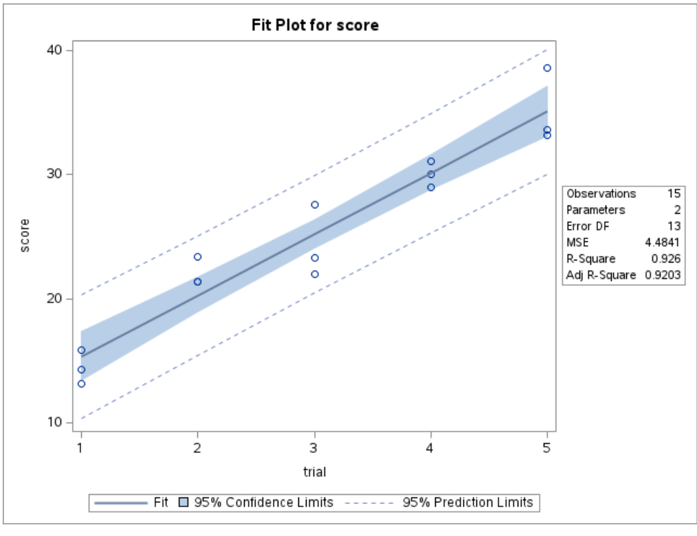
16.6.1 Step 1: A Model That Ignores Correlation
If we fit ordinary regression,
PROC REG DATA=performance;
    MODEL score = trial;
RUN;
QUIT;
this assumes all observations are independent.
That is not appropriate here, because repeated scores from the same person are likely correlated.
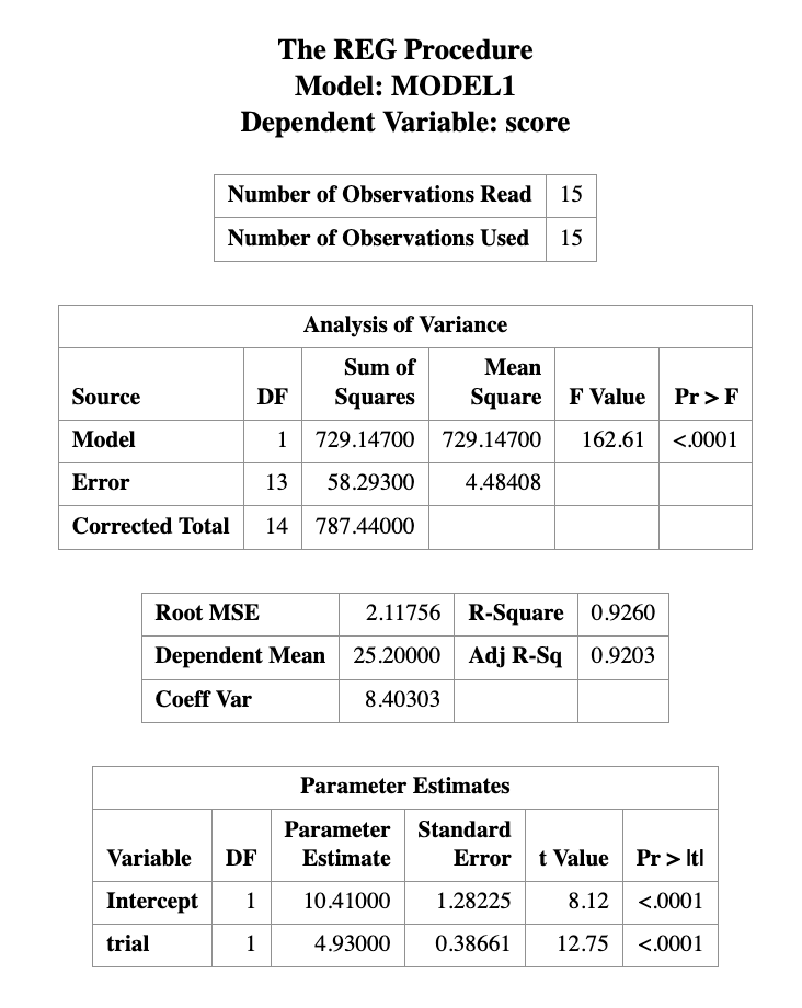
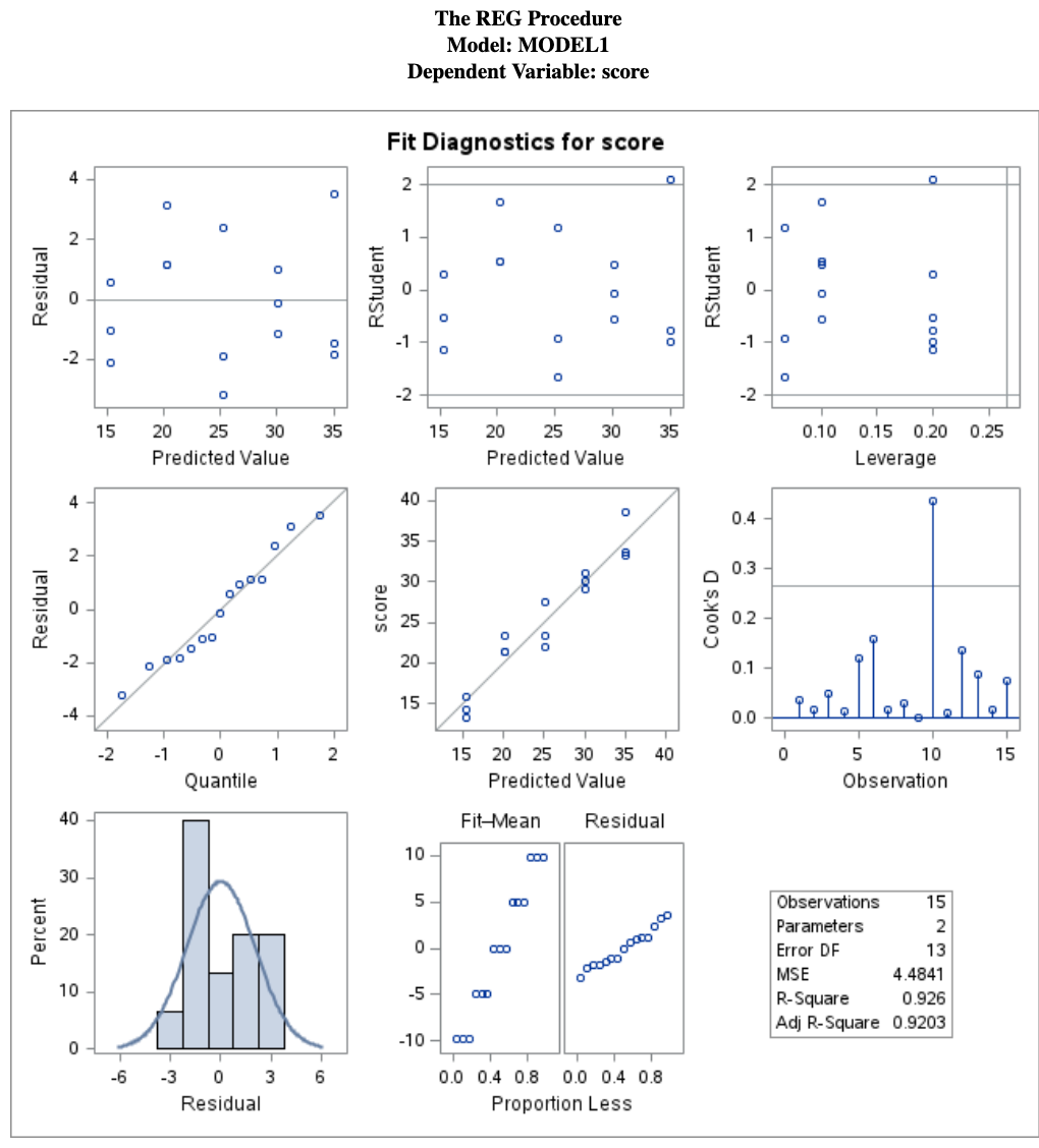
PROC REG is not designed for repeated-measures data with within-subject dependence.
It may still produce estimates, but the inference can be misleading because the independence assumption is violated.
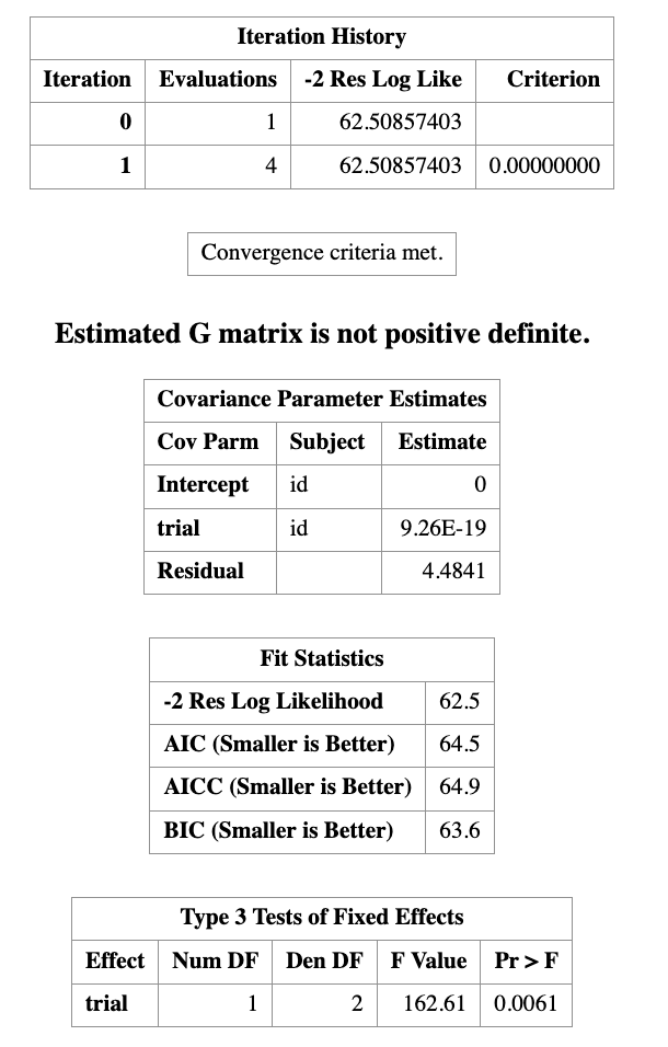
16.6.2 Step 2: Random Intercept Model
A natural first mixed model is the random intercept model.
PROC MIXED DATA=performance;
    CLASS id;
    MODEL score = trial;
    RANDOM INTERCEPT / SUBJECT=id;
RUN;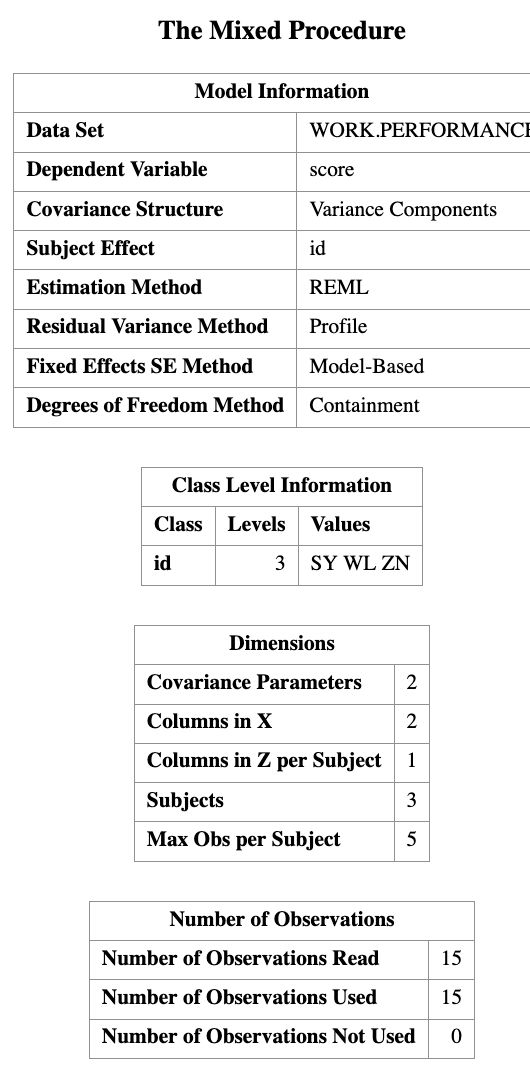
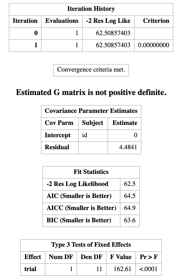
This corresponds to the model
\[ Y_{ij} = \beta_0 + \beta_1 \, trial_{ij} + u_i + \epsilon_{ij}. \]
Interpretation
- \(\beta_0\) is the overall intercept
- \(\beta_1\) is the average effect of trial
- \(u_i\) allows each subject to have their own baseline level
So this model says:
everyone follows the same overall slope, but each subject may start from a different intercept.
In the code above:
CLASS id;tells SAS thatidis a grouping variableMODEL score = trial;specifies the fixed-effects part of the modelRANDOM INTERCEPT / SUBJECT=id;tells SAS to fit a subject-specific random intercept
This is usually the first mixed model to try when each subject is observed multiple times.
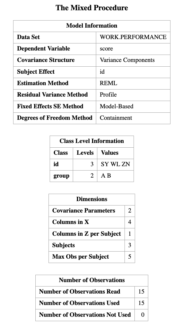
16.6.3 Step 3: Add Another Fixed Effect
We can also include group as a fixed effect.
PROC MIXED DATA=performance;
CLASS id group;
MODEL score = trial group;
RANDOM INTERCEPT / SUBJECT=id;
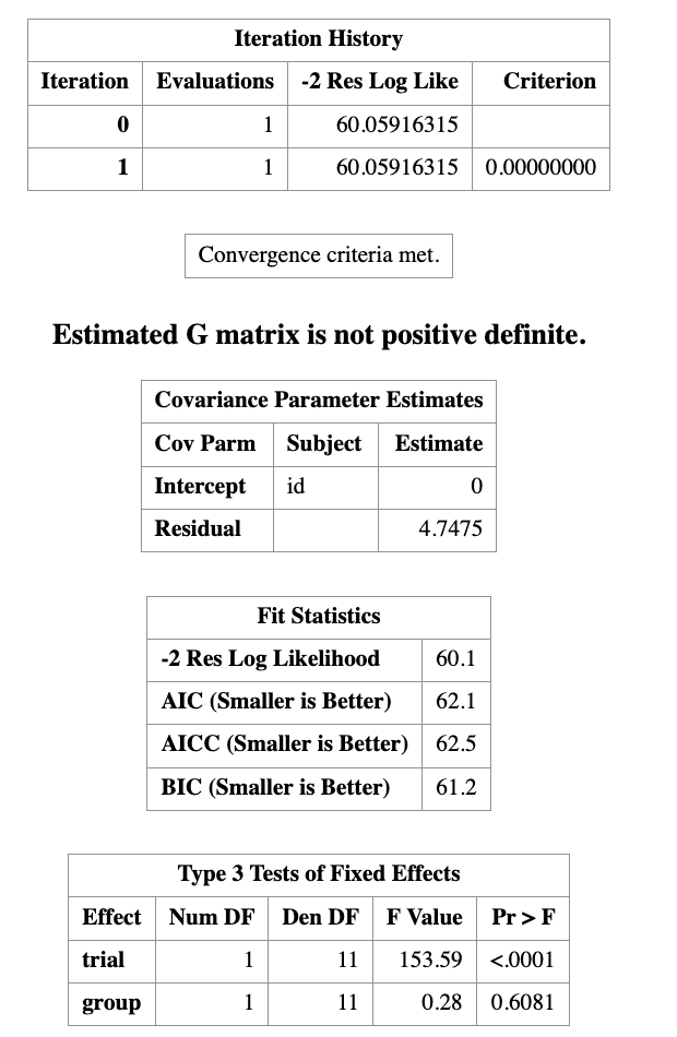
RUN;This corresponds to
\[ Y_{ij} = \beta_0 + \beta_1 \, trial_{ij} + \beta_2 \, group_{ij} + u_i + \epsilon_{ij}. \]
Now the model includes:
- an overall effect of trial
- an overall difference between groups
- a subject-specific random intercept
Intuition
trialasks whether scores tend to change over trialsgroupasks whether group A and group B differ on averageidas a random effect accounts for repeated measurements on the same subject
16.6.4 Step 4: Random Slope Model
A more flexible model allows the effect of trial to vary by subject.
PROC MIXED DATA=performance;
    CLASS id;
    MODEL score = trial;
    RANDOM INTERCEPT trial / SUBJECT=id;
RUN;
This corresponds to
\[ Y_{ij} = \beta_0 + \beta_1 trial_{ij} + u_{0i} + u_{1i} trial_{ij} + \epsilon_{ij}. \]
Interpretation
- \(u_{0i}\) allows subject \(i\) to have their own intercept
- \(u_{1i}\) allows subject \(i\) to have their own slope
This means different subjects can improve at different rates across trials.
- A random intercept model says subjects start at different levels
- A random slope model says subjects may also change at different rates
16.7 Conceptual Visualization
A helpful way to think about the difference between regression and mixed models is:
- ordinary regression: one fitted line for everyone
- random intercept model: many subject-specific lines with different intercepts
- random slope model: many subject-specific lines with different intercepts and different slopes
This is one reason mixed models are so useful for repeated-measures data.
16.8 In-Class Questions
Which variable is most appropriate as a random effect?
trial
score
id
group
Why include a random effect?
- To increase sample size
- To model dependence
- To remove variables
- To normalize the data
Ignoring clustering most directly leads to:
- Correct inference
- Smaller residuals
- Incorrect standard errors
- Better prediction
16.9 Summary of this class
This first lecture on linear mixed models is mainly about intuition.
The big picture is:
- Ordinary regression assumes independence
- Clustered and longitudinal data violate this assumption
- Random effects are used to model within-group dependence
- Mixed models combine:
- fixed effects for the mean structure
- random effects for the dependence structure
In the next lecture, we will go further into:
- more detailed interpretation of
PROC MIXEDoutput - covariance structures
- repeated-measures formulations
- model comparison and diagnostics
- Mixed models are used when observations are correlated
- Two common settings are:
- clustered data
- longitudinal data
- Fixed effects describe population-level effects
- Random effects describe subject- or cluster-specific deviations
- A random effect creates correlation among observations from the same subject or cluster
- In SAS, the most basic mixed model can be fitted using
PROC MIXED