1. Model the response and its uncertainty

Let \(x_i\) describe a candidate or experimental condition and \(y_i\) be its measured response. A simple working model is

\[ y_i = f(x_i) + \varepsilon_i,\qquad \varepsilon_i \overset{\mathrm{iid}}{\sim} N(0,\sigma^2). \]

Here \(f\) is the underlying response and \(\sigma^2\) represents measurement noise. The Gaussian noise assumption is illustrative; real assays may require another observation model.

A Gaussian process (GP) provides a predictive distribution for the latent response, conditional on observations \(\mathcal D_t=\{(x_i,y_i)\}_{i=1}^t\):

\[ f(x)\mid\mathcal D_t \sim N\!\left(\mu_t(x),s_t^2(x)\right). \]

The posterior mean \(\mu_t(x)\) estimates the response, while \(s_t(x)\) describes uncertainty about it under the chosen GP model. This is a standard statistical component of Bayesian optimization. [2]

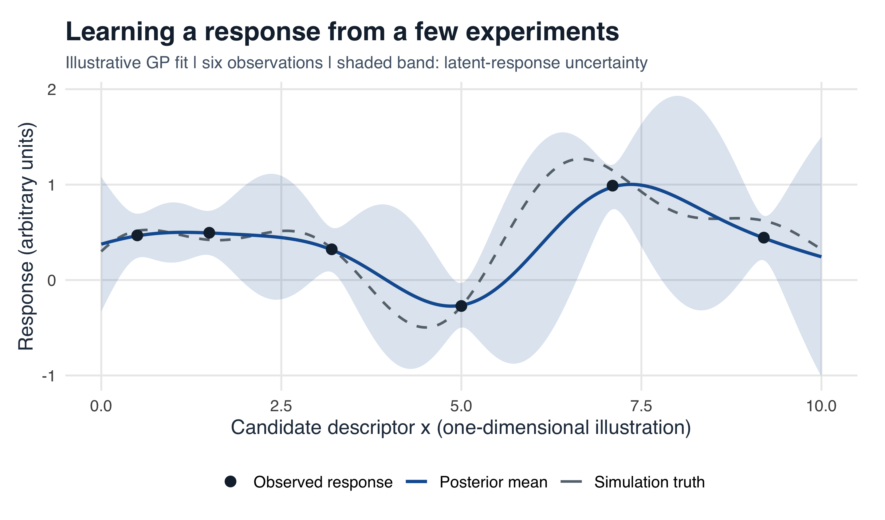
Figure 1: Simulated response learning. The blue band is a pointwise 95% posterior credible interval for the latent response, conditional on fixed GP hyperparameters. It is not a prediction interval for a new noisy measurement. The dashed curve is the simulation truth, available here only for illustration.

For a new measurement \(Y(x)\), the model-based predictive variance is \(s_t^2(x)+\sigma^2\). The distinction matters: uncertainty about an average response and variability in the next observation answer different questions.

2. Choose the next experiment

For an objective we want to maximize, expected improvement (EI) rewards candidates with a promising mean, useful uncertainty, or both. [2] With a fixed benchmark \(b_t\),

\[ \begin{aligned} \operatorname{EI}_t(x) &=\mathbb E[(f(x)-b_t)_+\mid\mathcal D_t] \\ &=(\mu_t(x)-b_t)\Phi(z_t(x))+s_t(x)\phi(z_t(x)),\\ z_t(x)&=\frac{\mu_t(x)-b_t}{s_t(x)}. \end{aligned} \]

Here \((u)_+=\max(u,0)\), and \(\Phi\) and \(\phi\) are the standard normal distribution and density functions. When \(s_t(x)=0\), EI is \(\max\{\mu_t(x)-b_t,0\}\). For this noisy illustration, \(b_t\) is the largest posterior mean among the tested candidates, a plug-in benchmark.

The next candidate on the search grid is

\[ x_{t+1}=\operatorname*{arg\,max}_{x\in\mathcal X} \operatorname{EI}_t(x). \]

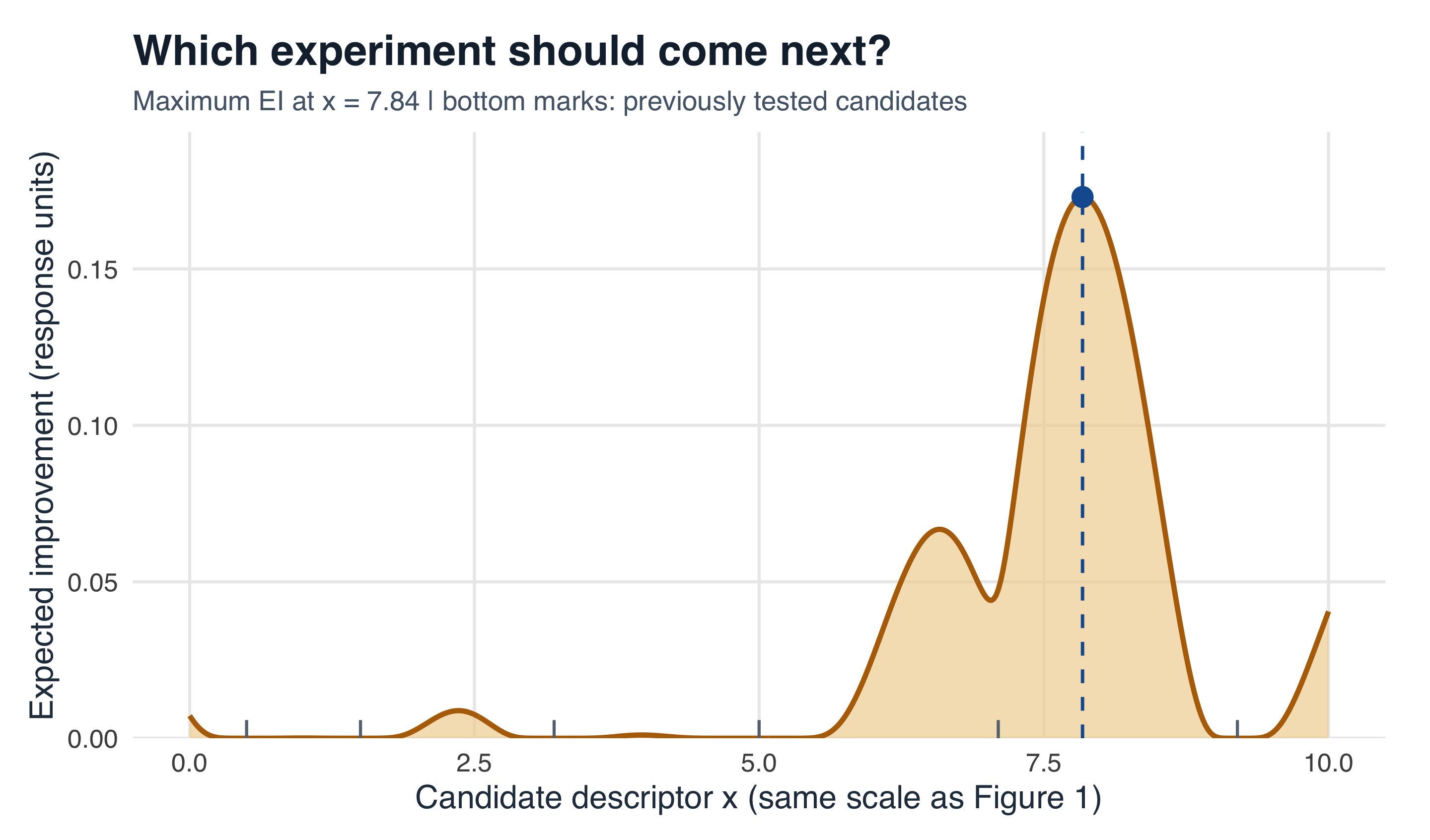
Figure 2: Expected improvement computed from the GP above. The marked maximum selects the next candidate on a fixed grid. This is one proposed next experiment, not evidence that the candidate is effective or safe.

In chemical synthesis, Shields et al. studied Bayesian optimization for selecting reaction conditions. [3] Drug-discovery decisions can involve additional objectives, such as toxicity, cost, or synthesizability; the single-response example here omits those constraints. See also the introduction to optimal regression design.

3. Calibrate intervals for future observations

Split conformal prediction calibrates a fixed predictor \(\widehat f\) using \(m\) held-out responses. Let \(r_i=|y_i-\widehat f(x_i)|\) and let \(r_{(k)}\) be their \(k\)th order statistic. [4]

\[ \begin{aligned} k&=\lceil(m+1)(1-\alpha)\rceil,\qquad \widehat q=r_{(k)},\\ C_\alpha(x)&=[\widehat f(x)-\widehat q,\; \widehat f(x)+\widehat q]. \end{aligned} \]

Set \(\widehat q=\infty\) if \(k>m\). When calibration and future observations are exchangeable, with the predictor fitted independently of calibration data,

\[ \Pr\{Y_{\mathrm{new}}\in C_\alpha(X_{\mathrm{new}})\} \geq 1-\alpha. \]

This is a marginal guarantee, not a guarantee for each compound or a fixed realized test sample. Adaptive candidate selection and shifts to a new chemical population can invalidate exchangeability and require additional methods. [4]

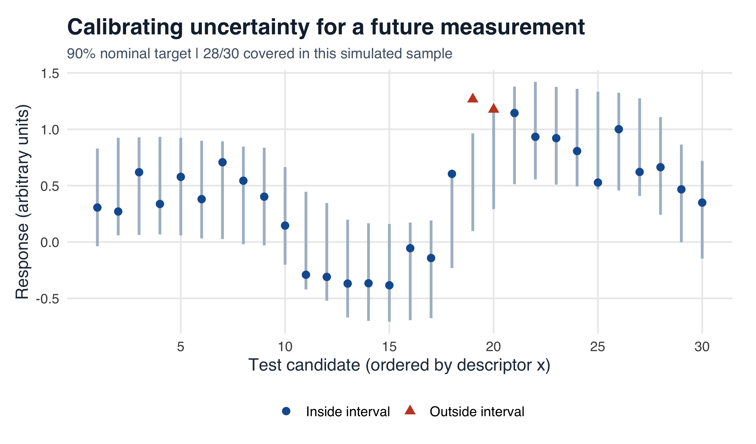
Figure 3: Prediction intervals for 30 simulated test observations, calibrated using 199 independent observations with a 90% nominal coverage target. Points are realized responses; triangles mark misses. This figure uses the same response-generating function as Figures 1–2 but an independent, non-adaptive test sample.

4. Connect the tools with an AI agent

An AI agent plans steps, calls tools, inspects their outputs, and revises its next action. Coscientist demonstrated an LLM-based system that connected tools for planning and performing chemical experiments. [5] Retrieval-augmented generation (RAG) can connect a language model to retrieved documents when generating an answer. [6]

A possible workflow is retrieve evidence → fit and check a model → propose an experiment → researcher review and measurement → update the data. The equations above belong to the statistical tools used within that workflow. A language model’s confident wording is not a substitute for a calibrated uncertainty estimate.

Research questions include how to preserve citations through retrieval, propagate uncertainty between tools, choose informative experiments under constraints, and evaluate an agent on reproducibility and scientific value. The proposed workflow connects statistical learning, optimal design, RAG, and LLM alignment.

References

1. U.S. Food and Drug Administration. Step 1: Discovery and development.
2. Snoek, J., Larochelle, H. & Adams, R. P. (2012). Practical Bayesian optimization of machine learning algorithms. Advances in Neural Information Processing Systems, 25.
3. Shields, B. J. et al. (2021). Bayesian reaction optimization as a tool for chemical synthesis. Nature, 590, 89–96.
4. Angelopoulos, A. N. & Bates, S. (2021). A gentle introduction to conformal prediction and distribution-free uncertainty quantification. arXiv:2107.07511.
5. Boiko, D. A., MacKnight, R., Kline, B. & Gomes, G. (2023). Autonomous chemical research with large language models. Nature, 624, 570–578.
6. Lewis, P. et al. (2020). Retrieval-augmented generation for knowledge-intensive NLP tasks. Advances in Neural Information Processing Systems, 33.

Notes and reproducibility

All three figures use simulated data in arbitrary units; they are teaching illustrations, not results from a drug-screening study.

All figures are generated from this article’s R Markdown source, using R and ggplot2 with fixed seeds. The GP uses a zero mean, a squared-exponential kernel with unit signal variance and length scale 1.1, and noise standard deviation 0.12. These are chosen teaching settings, not fitted biological parameters. The calibration sample and the 30 test points are generated independently after fixing the predictor; no test points were selected based on their outcomes.

The proposed agent workflow is a conceptual connection between these tools, not a validated drug-discovery system.