
Optimal regression design: an introduction
An illustrated introduction to optimal design for calibration, concentration-response experiments, group testing, and multiple objectives, with models, workflows, and reproducible R examples.
Which experimental settings should we use, and how often should we repeat each one? Optimal regression design answers this question by connecting a scientific goal to a statistical model and a limited experimental budget. The settings might be concentrations, sampling times, temperatures, or pool sizes. The goal might be precise parameter estimation, reliable response prediction, or learning a particular contrast.
The field combines statistical inference, matrix theory, and optimization. A design is optimal for a stated model, objective, and set of constraints; changing any of these can change the answer. Pukelsheim’s monograph develops the underlying theory. [1]
The examples below show how this translates into study plans:
- Laboratory calibration: where should 30 measurements be collected to learn an instrument response accurately?
- Concentration-response experiments: which concentrations make 60 assays informative about a compound’s half-maximal response?
- Prevalence surveys: how should pool size balance specimen costs, assay costs, and estimation precision?
- Multiple objectives: how much precision at a routinely used concentration can we gain while protecting estimation of the full response curve?
Each example specifies a model, compares feasible allocations, and quantifies a consequence for precision.
1. From a regression model to a design
Consider a regression that is linear in its unknown coefficients:
\[ \begin{aligned} Y_i&=f(x_i)^\top\beta+\varepsilon_i,\\ \mathbb E(\varepsilon_i)&=0,\qquad \operatorname{Var}(\varepsilon_i)=\sigma^2. \end{aligned} \]
Assume independent errors, a known regression basis \(f(x)\in\mathbb R^p\), and a controllable setting \(x\) in a feasible region \(\mathcal X\). Throughout, vectors are column vectors. For quadratic regression, write the basis directly as
\[ f(x)=\begin{pmatrix}1\\x\\x^2\end{pmatrix}. \]
The model is still linear in the parameters even though its response curve can bend. Transposes below indicate inner products or matrix products.
An approximate design records support points and allocation proportions:
\[ \begin{gathered} \xi=\{(x_1,w_1),\ldots,(x_k,w_k)\},\\ w_j\geq0,\quad\sum_{j=1}^k w_j=1. \end{gathered} \]
For \(N\) observations, an exact design instead specifies integer replication counts \(n_j\) with \(\sum_j n_j=N\). Its proportions are \(w_j=n_j/N\). Approximate designs let us optimize continuously; implementing them requires integer allocations. Rounding and exact-design optimization are substantive parts of the problem. [2]
Define the normalized information matrix
\[ M(\xi)=\sum_{j=1}^k w_j f(x_j)f(x_j)^\top. \]
When \(M(\xi)\) is nonsingular and the allocations are realized exactly, ordinary least squares gives
\[ \operatorname{Cov}(\widehat\beta)=\frac{\sigma^2}{N}M(\xi)^{-1}. \]
This covariance identity needs the stated mean and variance assumptions, not Gaussian errors. With Gaussian errors, the Fisher information for \(\beta\) is \(N M(\xi)/\sigma^2\). A singular matrix means that the full coefficient vector cannot be identified from that design.
2. Match the criterion to the scientific question
The usual criteria summarize different aspects of information. In the table, \(M=M(\xi)\) is nonsingular, \(c\) is a specified contrast vector, and \(\nu\) is a chosen probability measure describing where prediction matters. [1]
| Criterion | Optimization target | Scientific emphasis |
|---|---|---|
| D | Maximize \(\log\det M\) | Joint precision of all coefficients; smaller confidence ellipsoid under the usual Gaussian or asymptotic approximation. |
| A | Minimize \(\operatorname{tr}(M^{-1})\) | Total coefficient variance on the chosen parameter scale. |
| E | Maximize \(\lambda_{\min}(M)\) | Protect the least precisely estimated unit-length coefficient direction. |
| c | Minimize \(c^\top M^{-1}c\) | Precision of the particular quantity \(c^\top\beta\). |
| G | Minimize \(\max_{x\in\mathcal X} f(x)^\top M^{-1}f(x)\) | Worst-case variance of the estimated mean response over the design region. |
| I | Minimize \(\int f(x)^\top M^{-1}f(x)\,d\nu(x)\) | Average mean-response variance over a target region or population. |
For example, estimating curvature suggests a contrast involving the quadratic coefficient; predicting throughout an operating range suggests a prediction criterion. A- and E-optimality depend on parameter scaling. D-optimal designs are invariant to a fixed nonsingular linear reparameterization. For c-optimality, singular designs can also be admissible when the specified contrast remains estimable; that requires a generalized-inverse formulation.
3. Laboratory calibration: get more precision from 30 measurements
The decision. A laboratory has already checked that a quadratic model adequately describes its instrument response over concentrations \(z\in[0,100]\,\mu\mathrm M\). It now plans a focused follow-up experiment with 30 independent measurements to estimate that curve more precisely. Calibration relates known reference quantities to instrument responses; the choice of model is consequential for subsequent measurement. [9]
Use the coded concentration \(x=(z-50)/50\) and the model
\[ Y=\beta_0+\beta_1x+\beta_2x^2+\varepsilon. \]
The intercept describes the mean signal at the center of the range; the other coefficients describe its slope and curvature on the coded scale. Assume constant error variance and compare two allocations with the same \(N=30\):
- Equally spaced: one measurement at each of 30 concentrations spanning 0 to 100 \(\mu\mathrm M\).
- D-optimal: ten independent measurements each at 0, 50, and 100 \(\mu\mathrm M\), corresponding to \(x=-1,0,1\).
The second allocation corresponds to \(\xi_D=\{(-1,1/3),(0,1/3),(1,1/3)\}\). Here the approximate optimum is exactly implementable because 30 is divisible by three. Section 7 verifies optimality over the entire interval.
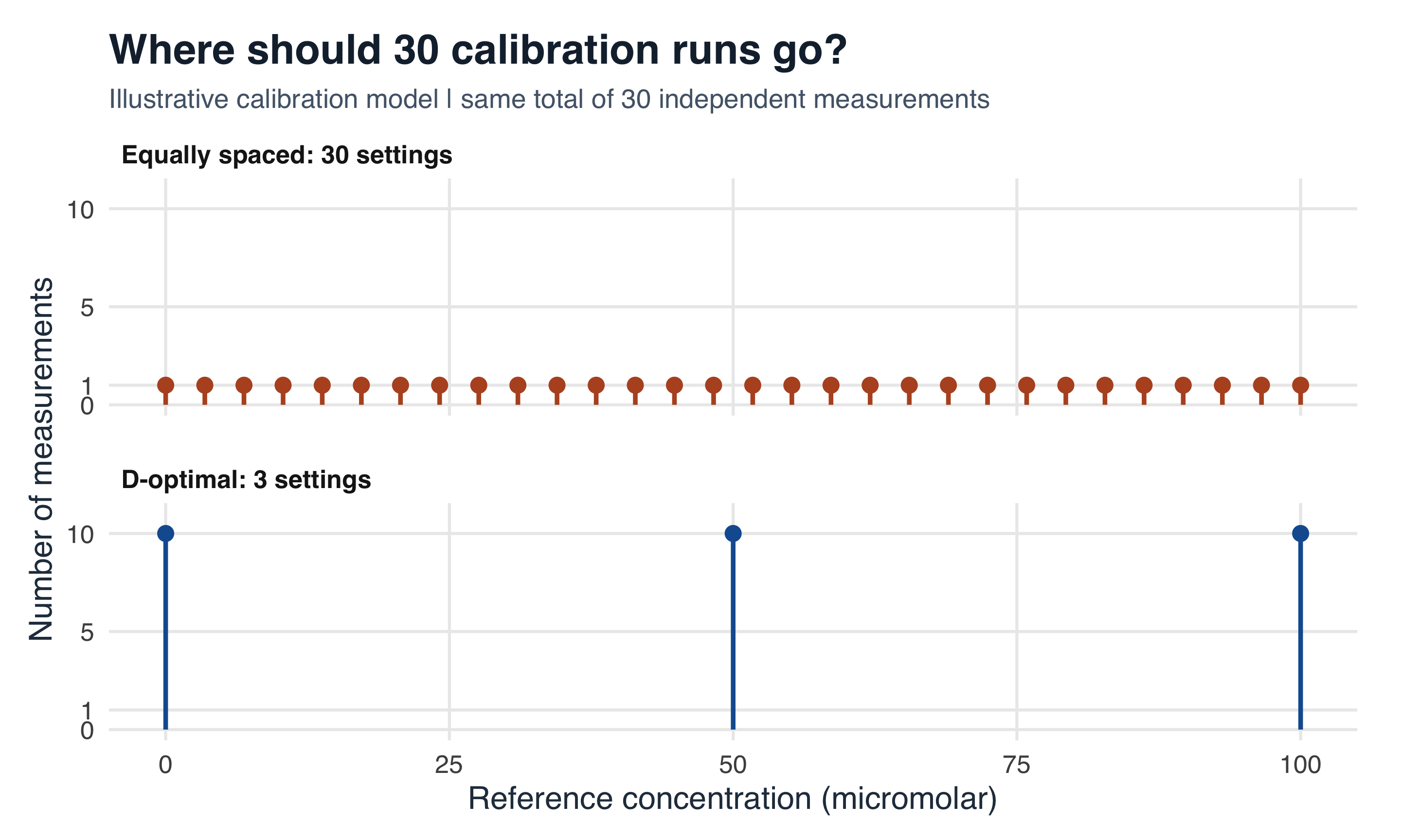
Figure 1: Figure 1. Two allocations of the same 30 observations. Height gives the number of independent observations at each setting. Replication at three carefully chosen locations is sufficient for the assumed three-parameter quadratic model.
To compare prediction precision, write \(\widehat m(x)=f(x)^\top\widehat\beta\). Then
\[ \begin{aligned} \operatorname{Var}\{\widehat m(x)\} &=\frac{\sigma^2}{N}\,d(x,\xi),\\ d(x,\xi)&=f(x)^\top M(\xi)^{-1}f(x). \end{aligned} \]
The curves below show \(d(x,\xi)\), so they do not require selecting a noise variance. Predicting an independent new observation, rather than its mean, adds \(\sigma^2\) to the displayed variance after rescaling.
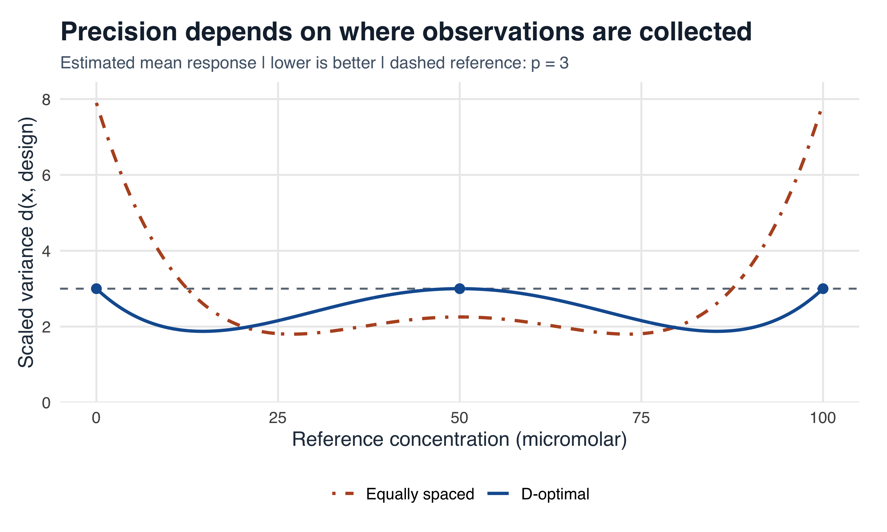
Figure 2: Figure 2. Scaled variance of the estimated mean response, computed directly from each design matrix. Multiply the vertical axis by sigma squared / 30 to obtain the mean-estimation variance. The dashed line at p = 3 is the D/G-optimality bound for this unconstrained linear-model problem.
A useful summary is D-efficiency relative to the optimum:
\[ \operatorname{Eff}_D(\xi) =\left\{\frac{\det M(\xi)}{\det M(\xi_D)}\right\}^{1/p}. \]
| Design | Distinct settings | D-efficiency | Maximum scaled variance |
|---|---|---|---|
| Equally spaced | 30 | 62.4% | 7.899 |
| D-optimal | 3 | 100.0% | 3.000 |
Why this matters. If the instrument noise standard deviation is 2 signal units, the worst-case standard error of the estimated mean signal falls from 1.026 to 0.632, about 38.4% lower, using the same 30 measurements. The design also uses three distinct reference concentrations instead of thirty. These SEs concern the forward mean signal; uncertainty in an unknown concentration inferred by inverting the curve is a different design target.
This is a focused estimation design after model validation. Three distinct settings leave no lack-of-fit degrees of freedom beyond the quadratic mean model. If checking departures from quadratic behavior matters, allocate observations to additional settings or optimize a criterion that explicitly includes model checking.
4. Concentration-response experiments: spend wells where the curve is informative
The decision. A laboratory has 60 independent assay runs for learning a compound’s concentration-response curve between 0 and 100 \(\mu\mathrm M\). Estimating the half-maximal concentration can help compare compounds and plan the next assay range. Measurements all near a plateau provide little information about where the curve starts to rise.
A useful saturating model is the Emax model [10]:
\[ \begin{aligned} Y_i&=E_0+E_{\max}\frac{d_i}{K+d_i}+\varepsilon_i,\\ \varepsilon_i&\overset{\mathrm{iid}}{\sim}N(0,\sigma^2). \end{aligned} \]
Here \(d\) is concentration, \(E_0\) is baseline response, \(E_{\max}\) is the increase above baseline at saturation, and \(K\) is the concentration giving half that increase, often called \(EC_{50}\). Assume pilot information suggests \(E_0=10\), \(E_{\max}=80\), \(K=20\,\mu\mathrm M\), and \(\sigma=5\) signal units. These are chosen planning values for a hypothetical laboratory assay.
For the parameter vector \(\theta\), the gradient is a column vector:
\[ \theta=\begin{pmatrix}E_0\\E_{\max}\\K\end{pmatrix}, \qquad h(d;\theta)=\begin{pmatrix} 1\\[2pt] \dfrac{d}{K+d}\\[4pt] -\dfrac{E_{\max}d}{(K+d)^2} \end{pmatrix}. \]
With \(n_j\) runs at concentration \(d_j\), the local information approximation gives
\[ \operatorname{Cov}(\widehat\theta) \approx\sigma^2\left\{\sum_j n_j h(d_j;\theta)h(d_j;\theta)^\top\right\}^{-1}. \]
Compare two plans. The baseline uses ten runs at each of 0, 20, 40, 60, 80, and 100 \(\mu\mathrm M\). With an upper concentration \(D=100\), the local D-optimal plan uses equal allocation at
\[ d_1=0,\qquad d_2=\frac{DK}{D+2K},\qquad d_3=D. \]
Thus, allocate twenty runs each at 0, approximately 14.29, and 100 \(\mu\mathrm M\). One way to derive this result is to transform concentration to \(t=d/(K+d)\). The three gradient components span a quadratic basis in \(t\), whose D-optimal support consists of the two endpoints and their midpoint. Equal spacing on this transformed scale is not equal spacing in concentration.
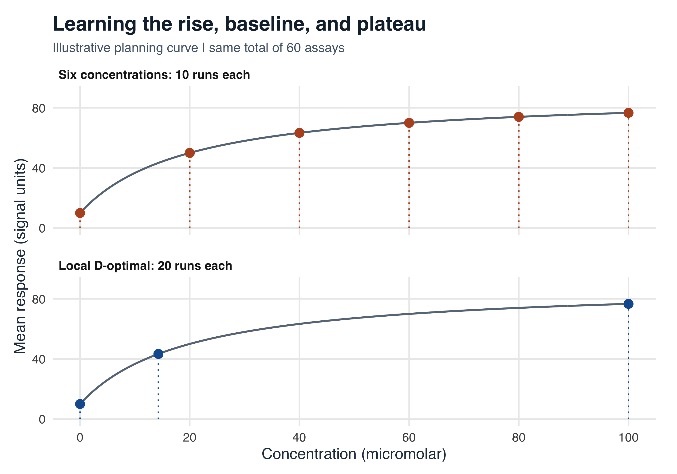
Figure 3: Figure 3. A hypothetical Emax response curve and two ways to allocate 60 independent assays. Dots lie on the assumed planning curve; they are not measured outcomes. Each dot represents 10 runs in the upper panel or 20 runs in the lower panel. The local design depends on the assumed K = 20 micromolar.
| Parameter | Baseline SE | Local design SE |
|---|---|---|
| Baseline E0 (signal units) | 1.58 | 1.12 |
| Maximum increase Emax (signal units) | 2.99 | 2.31 |
| Half-maximal concentration K (micromolar) | 2.66 | 1.97 |
Why this matters. Under these planning assumptions, the approximate standard error for \(K\) falls from 2.66 to 1.97 \(\mu\mathrm M\), a 25.8% reduction, with no increase in assay count. These are local Fisher-information planning SEs. The design optimizes joint parameter precision; if only \(K\) matters, a c-optimal criterion targets that question directly.
A practical plan would assess several plausible \(K\) values, allow additional concentrations for model checking, and account for plate or batch effects. A changed \(K\), concentration-dependent noise, or a sigmoidal rather than Emax response changes the preferred design. Independent replication and randomized run order help separate the concentration response from laboratory drift.
5. Group testing: balance assay cost against prevalence precision
The decision. A prevalence survey can combine specimens into pools and record whether each pooled assay is positive. The aim is to estimate the population prevalence, rather than identify every positive individual. Pool size changes both the chance of a positive assay and the cost of obtaining that information. This is the setting of group-testing design research. [11] [8]
Assume independently sampled specimens with prevalence \(\pi\), disjoint pools of size \(s\), assay sensitivity \(\mathrm{Se}\), and specificity \(\mathrm{Sp}\). Define \(a_s=(1-\pi)^s\), the probability that a pool contains no positive specimens. Then
\[ \begin{aligned} q_s(\pi)&=\mathrm{Se}(1-a_s)+(1-\mathrm{Sp})a_s,\\ Z_s&\sim\operatorname{Binomial}(n_s,q_s(\pi)), \end{aligned} \]
where \(Z_s\) counts positive assays among \(n_s\) pools. For this first calculation, take sensitivity and specificity as known and constant across pool sizes. The information per pooled assay about \(\pi\) is
\[ \begin{aligned} q_s'(\pi)&=s(\mathrm{Se}+\mathrm{Sp}-1)(1-\pi)^{s-1},\\ I_s(\pi)&=\frac{\{q_s'(\pi)\}^2}{q_s(\pi)\{1-q_s(\pi)\}},\\ \operatorname{SE}(\widehat\pi)&\approx\{n_s I_s(\pi)\}^{-1/2}. \end{aligned} \]
A budgeted illustration. Suppose the planning prevalence is 2%, sensitivity is 95%, and specificity is 99%. Use a hypothetical budget of 5,000 cost units, with 20 units per pooled assay plus 1 per specimen, including the modeled collection and preparation cost. For a plan using a single pool size,
\[ n_s=\left\lfloor\frac{5000}{20+s}\right\rfloor, \qquad s\in\{1,\ldots,50\}. \]
All plans below respect the same total budget. They differ in both the number of assays and the number of specimens collected.
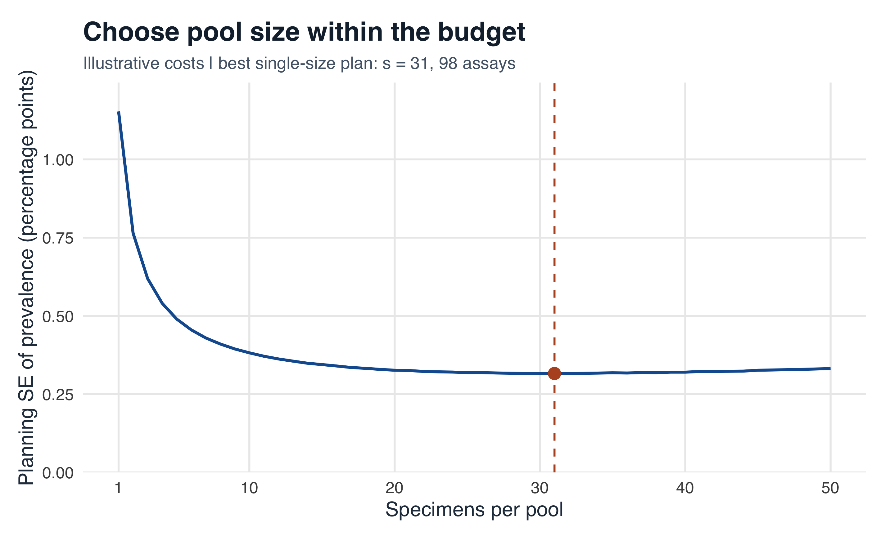
Figure 4: Figure 4. Approximate prevalence-estimation standard error for each single-pool-size plan under a 5,000-unit budget. The highlighted minimum is over integer sizes 1 to 50 only; mixed-size plans were not optimized. Sensitivity and specificity are assumed known, with no dilution effect. Values are calculated at a 2% planning prevalence.
| Pool size | Assays | Specimens | SE (percentage points) |
|---|---|---|---|
| 1 | 238 | 238 | 1.153 |
| 10 | 166 | 1660 | 0.382 |
| 31 | 98 | 3038 | 0.316 |
| 50 | 71 | 3550 | 0.332 |
Why this matters. Individual testing spends almost all of this budget on assays and gives a planning SE of 1.153 percentage points. The best single-size plan in this comparison uses 98 pools of 31, covering 3038 specimens, with an SE of 0.316 percentage points. Collecting more specimens is explicitly charged to the budget. The calculation illustrates how optimizing information per unit cost can change the study plan; it does not establish 31 as a generally preferred pool size.
For implementation, specify dilution-dependent sensitivity, specimen availability, overhead, and any individual follow-up testing that the study requires. If sensitivity and specificity must also be estimated, one pool size supplies only one positive-assay probability for three unknowns. It cannot identify all three parameters. Multiple pool sizes or external validation data are then needed, leading naturally to the multi-parameter and multi-objective designs in the gtDesign research. [11] [8]
6. Multi-objective design: protect the curve and improve a routine measurement
The decision. Return to the quadratic calibration experiment in Section 3. Suppose the laboratory routinely checks samples at 50 \(\mu\mathrm M\), but still needs to estimate the response curve across the full 0–100 range. Its 30 measurements now serve two purposes:
- Joint parameter precision: estimate the intercept, slope, and curvature using a D-criterion.
- Precision at the routine concentration: estimate the mean signal at 50 \(\mu\mathrm M\), where \(x=0\) and \(m(0)=\beta_0\), using a c-criterion with \(c=\begin{pmatrix}1\\0\\0\end{pmatrix}\).
These goals favor different allocations. A D-optimal plan spreads replication evenly across the three settings; estimating only the center mean would put every measurement at the center and leave slope and curvature unidentified. Multi-objective design makes the compromise explicit. Compound criteria combine objectives using priorities; constrained criteria instead specify a minimum acceptable efficiency for one objective and optimize the other. [12]

A transparent model for the trade-off
For this illustration, restrict attention to symmetric allocations at 0, 50, and 100 \(\mu\mathrm M\). Let \(u\) be the total fraction at the two endpoints, so the coded design is
\[ \begin{gathered} \xi(u)=\{(-1,u/2),(0,1-u),(1,u/2)\},\\ 0<u<1,\qquad M(u)=\begin{pmatrix} 1&0&u\\ 0&u&0\\ u&0&u \end{pmatrix}. \end{gathered} \]
Direct calculation gives \(\det M(u)=u^2(1-u)\) and \(c^\top M(u)^{-1}c=1/(1-u)\). Normalize each objective by its own single-objective optimum:
\[ \begin{aligned} \operatorname{Eff}_D(u) &=\left\{\frac{27}{4}u^2(1-u)\right\}^{1/3},\\ \operatorname{Eff}_c(u)&=1-u,\\ \operatorname{SE}\{\widehat m(0)\} &=\frac{\sigma}{\sqrt{N(1-u)}}. \end{aligned} \]
The D-efficiency reference is the equal-allocation design, \(u=2/3\). The c-efficiency reference is the all-center design: it estimates the center mean with variance \(\sigma^2/N\) even though its full information matrix is singular. Both efficiencies are dimensionless; higher is better. The displayed SE concerns the estimated mean, not a future noisy observation or an inversely estimated concentration.
One compound criterion is a weighted sum of log efficiencies:
\[ \begin{gathered} \max_{0<u<1}\;\Phi_\lambda(u),\\ \begin{aligned} \Phi_\lambda(u) &=\lambda\log\operatorname{Eff}_D(u)\\ &\quad +(1-\lambda)\log\operatorname{Eff}_c(u), \end{aligned} \end{gathered} \]
where \(0<\lambda\leq1\) encodes the chosen priority on joint precision. It is not the fraction of the budget spent on that objective. Differentiation yields
\[ \begin{aligned} \Phi_\lambda'(u) &=\frac{2\lambda}{3u} -\frac{1-2\lambda/3}{1-u},\\ u_\lambda&=\frac{2\lambda}{3}. \end{aligned} \]
The criterion is strictly concave in \(u\), so this is its unique optimum in the stated family. At \(\lambda=1\) it recovers the D-optimal allocation; smaller positive weights move measurements toward the center. As \(\lambda\) tends to zero, the design tends to the singular all-center reference. This derivation is specific to the quadratic model, the center target, and the allowed symmetric three-setting plans.
What would the laboratory actually run?
Keep \(N=30\) and \(\sigma=2\) signal units. These three compound designs have exact integer allocations, so no rounding is needed:
| Plan | \(\lambda\) | Runs at 0 / 50 / 100 | D-efficiency | Center SE | Endpoint SE |
|---|---|---|---|---|---|
| D-optimal | 1.0 | 10 / 10 / 10 | 100.0% | 0.632 | 0.632 |
| Compromise | 0.8 | 8 / 14 / 8 | 96.4% | 0.535 | 0.707 |
| Center emphasis | 0.5 | 5 / 20 / 5 | 79.4% | 0.447 | 0.894 |
Both SE columns use signal units; the endpoint value applies at either 0 or 100 \(\mu\mathrm M\). The 8 / 14 / 8 compromise retains 96.4% D-efficiency while reducing the center SE from 0.632 to 0.535, a 15.5% reduction. The cost is visible: each endpoint SE increases from 0.632 to 0.707. A small loss of D-efficiency does not mean that every individual variance changes by the same small percentage.
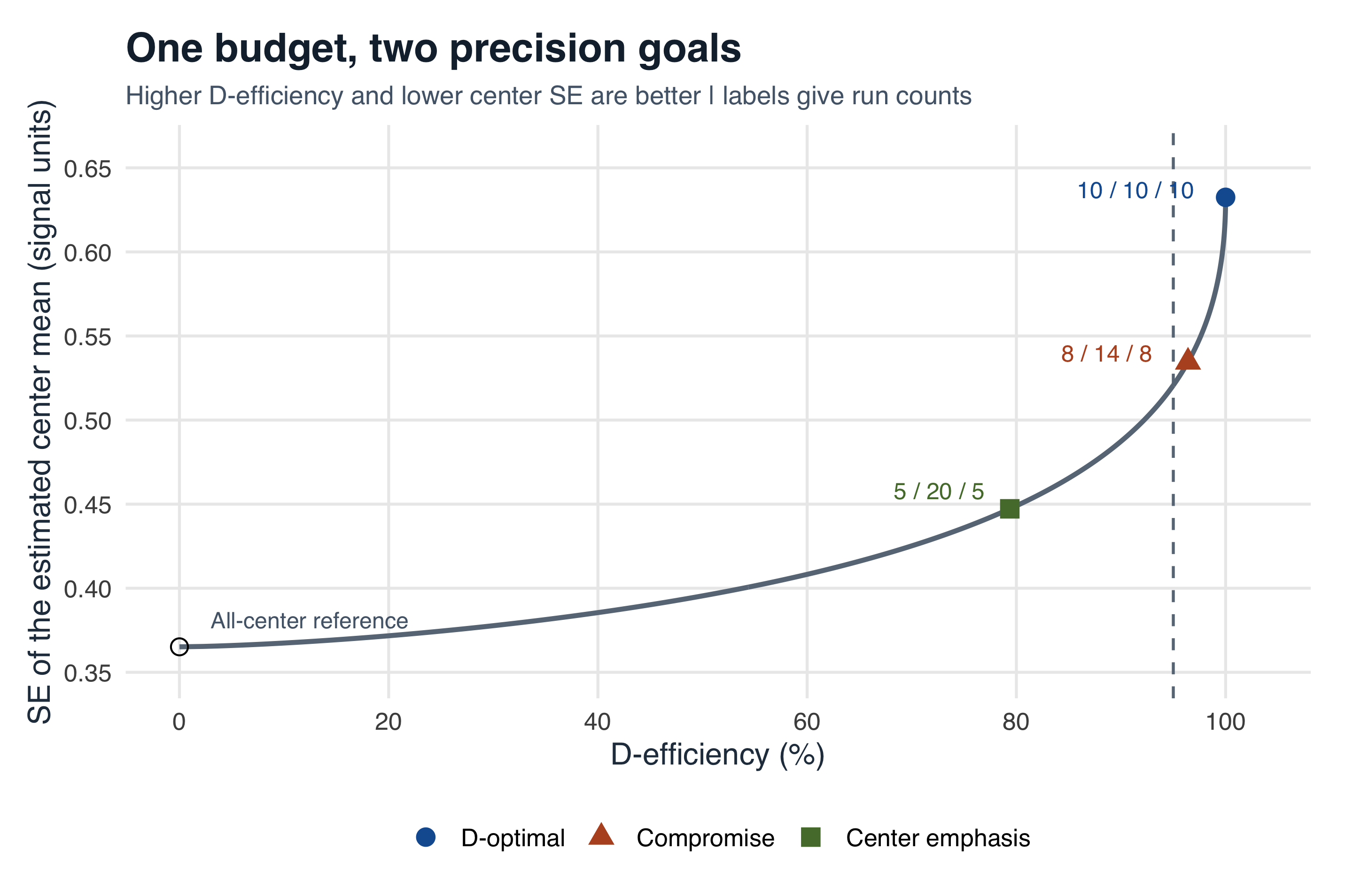
Figure 5: Figure 5. The Pareto trade-off within symmetric three-setting calibration designs with 30 runs and noise SD 2. Higher D-efficiency and lower center SE are preferred. The continuous curve uses approximate allocations; the highlighted plans have integer run counts. The dashed line marks a 95% D-efficiency requirement. The all-center endpoint is a singular reference that cannot estimate the full curve.
The curve is a Pareto frontier within this design family: for \(0<u\leq2/3\), improving joint efficiency worsens precision at the center. Values \(u>2/3\) are dominated by the D-optimal plan because they worsen both objectives. The frontier helps choose a scientifically acceptable compromise; it does not select the priorities for the researcher.
Choose an efficiency requirement instead of a weight
A laboratory may find the requirement “retain at least 95% D-efficiency, then minimize the center SE” easier to justify than choosing \(\lambda\). For an exact symmetric plan, put \(k\) observations at each endpoint and \(30-2k\) at the center:
\[ \begin{gathered} \min_{k\in\{1,\ldots,14\}} \frac{2}{\sqrt{30-2k}}\\ \text{subject to}\quad \operatorname{Eff}_D(2k/30)\geq0.95. \end{gathered} \]
Enumerating these fourteen feasible full-rank allocations gives \(k=8\), hence 8 / 14 / 8 again. This is the best center precision subject to the 95% requirement among these symmetric integer plans, rather than an unverified claim over arbitrary locations or other experimental constraints.
R code: multi-objective design
# Standalone base-R example: 30 runs at 0, 50, and 100 micromolar.
multi_N <- 30
multi_sigma <- 2
multi_D_eff <- function(u) ((27 / 4) * u^2 * (1 - u))^(1 / 3)
multi_center_se <- function(u) multi_sigma / sqrt(multi_N * (1 - u))
multi_score <- function(u, lambda) {
  lambda * log(multi_D_eff(u)) + (1 - lambda) * log(1 - u)
}

# u is the total fraction assigned to the two endpoints.
# The analytic compound optimum is u = 2 * lambda / 3.
multi_lambda <- c(1, 0.8, 0.5)
multi_u <- 2 * multi_lambda / 3
multi_choices <- data.frame(
  plan = c('D-optimal', 'Compromise', 'Center emphasis'),
  lambda = multi_lambda,
  u = multi_u,
  n0 = round(multi_N * multi_u / 2),
  n50 = round(multi_N * (1 - multi_u)),
  n100 = round(multi_N * multi_u / 2),
  D_eff = multi_D_eff(multi_u),
  center_se = multi_center_se(multi_u),
  endpoint_se = multi_sigma / sqrt(multi_N * multi_u / 2))

# Search all full-rank, symmetric integer allocations on these settings.
multi_integer <- data.frame(n_end = 1:14)
multi_integer$u <- 2 * multi_integer$n_end / multi_N
multi_integer$D_eff <- multi_D_eff(multi_integer$u)
multi_integer$center_se <- multi_center_se(multi_integer$u)
multi_feasible <- subset(multi_integer, D_eff >= 0.95)
multi_best <- multi_feasible[which.min(multi_feasible$center_se), ]

# Independently check the formulas against regression information matrices.
multi_F <- cbind(1, c(-1, 0, 1), c(1, 0, 1))
for (i in seq_along(multi_lambda)) {
  u <- multi_u[i]
  M <- crossprod(sweep(multi_F, 1, sqrt(c(u / 2, 1 - u, u / 2)), '*'))
  V <- multi_sigma^2 / multi_N * solve(M)
  numeric_u <- optimize(function(v) -multi_score(v, multi_lambda[i]),
                        c(1e-6, 1 - 1e-6), tol = 1e-10)$minimum
  stopifnot(abs(det(M) - u^2 * (1 - u)) < 1e-12,
            abs(sqrt(V[1, 1]) - multi_choices$center_se[i]) < 1e-10,
            abs(numeric_u - u) < 1e-6)
}
stopifnot(all(with(multi_choices, n0 + n50 + n100) == multi_N),
          multi_best$n_end == 8)
multi_choices
The same idea extends to screening studies. When prevalence, sensitivity, and specificity all need estimation, form efficiencies for those separate targets and choose either scientific priority weights or minimum acceptable efficiencies. Recompute the information matrix, account for assay and specimen costs, and check identifiability. The calibration formulas above do not carry over unchanged; this is where multi-objective group-testing methods become useful. [8]
7. Verify optimality with an equivalence theorem
For an unconstrained approximate design in a full-rank linear model with continuous \(f\) on compact \(\mathcal X\), the Kiefer–Wolfowitz equivalence theorem connects D-optimality, G-optimality, and the sensitivity bound [3]:
\[ \xi^*\text{ is D-optimal} \quad\Longleftrightarrow\quad \max_{x\in\mathcal X}d(x,\xi^*)=p. \]
At support points carrying positive weight, \(d(x,\xi^*)=p\). Intuitively, no feasible location offers a positive first-order improvement in log-determinant information when a small amount of allocation is moved there. The general theory extends beyond D-optimality. [1]
For our proposed quadratic design, direct matrix inversion gives
\[ \begin{gathered} M(\xi_D)= \begin{pmatrix} 1&0&2/3\\ 0&2/3&0\\ 2/3&0&2/3 \end{pmatrix},\\[4pt] d(x,\xi_D)=3-\frac{9}{2}x^2(1-x^2)\leq3. \end{gathered} \]
The inequality holds for every \(x\in[-1,1]\), with equality at \(-1,0,1\). This is an analytic certificate of optimality, not just a successful numerical search. In more complicated problems, evaluating sensitivity on a dense grid is a useful diagnostic but does not certify a continuous region unless the gaps between grid points are also controlled. Added cost or allocation constraints require the corresponding constrained optimality conditions.
8. Computing a design
On a fixed candidate set \(x_1,\ldots,x_m\), information is affine in the weights. For example, D-optimality solves
\[ \max_{w\geq0,\;\mathbf1^\top w=1} \log\det\!\left\{\sum_{j=1}^m w_j f(x_j)f(x_j)^\top\right\}. \]
This is convex optimization in the standard sense of maximizing a concave objective over a convex feasible set. Linear restrictions on allocation can be included. E-optimality also has a semidefinite formulation: maximize \(t\) subject to \(M(w)-tI_p\succeq0\) and the weight constraints. Integer run counts and freely moving support locations introduce additional computational issues. [2]
Exchange algorithms modify support points or allocations; conic optimization provides another route. CVXR lets R users express supported convex objectives and constraints and pass them to numerical solvers. [4] Regardless of the algorithm, inspect feasibility, matrix rank, sensitivity, and the efficiency of the final integer allocation.
9. Beyond ordinary linear regression
For independent observations from a parametric model, replace the outer product \(f(x)f(x)^\top\) by the appropriate per-observation Fisher information \(I(x;\theta)\). In homoscedastic Gaussian nonlinear regression with mean \(g(x;\theta)\),
\[ \begin{aligned} I(x;\theta)&=\frac{1}{\sigma^2} \nabla_\theta g(x;\theta)\nabla_\theta g(x;\theta)^\top,\\ M(\xi;\theta)&=\sum_j w_j I(x_j;\theta). \end{aligned} \]
For logistic regression, \(I(x;\beta)=\pi(x)\{1-\pi(x)\}f(x)f(x)^\top\), with \(\pi(x)=\operatorname{logit}^{-1}\{f(x)^\top\beta\}\). The information now depends on unknown parameters, making design and prior scientific knowledge closely connected. Atkinson & Woods review design for generalized linear models. [5]
- Local design: optimize at a nominal parameter value supported by prior evidence.
- Prior-averaged design: average an information criterion over a specified parameter distribution.
- Maximin design: protect performance across a scientifically chosen parameter set.
- Sequential design: update parameter estimates or distributions after an initial stage and redesign subsequent stages.
For example, two information-based objectives are
\[ \begin{gathered} \max_\xi\int\log\det M(\xi;\theta)\,d\Pi(\theta),\\[4pt] \max_\xi\min_{\theta\in\Theta} \operatorname{Eff}_D(\xi;\theta). \end{gathered} \]
In the second expression, efficiency is relative to the local optimum at each \(\theta\). The first is often called pseudo-Bayesian D-optimality; it is distinct from a fully Bayesian expected-utility calculation that averages over future data and posterior decisions. [6]
Uncertainty about parameters also differs from model misspecification. If the assumed mean or variance structure is wrong, evaluate the resulting bias and covariance under explicit alternatives. A mean squared error criterion combines both:
\[ \operatorname{MSE}(\widehat\beta) =\operatorname{Cov}(\widehat\beta) +\operatorname{Bias}(\widehat\beta)\operatorname{Bias}(\widehat\beta)^\top. \]
The target parameter and the allowed departures from the model must be defined before a worst-case MSE problem is meaningful.
10. From these examples to a research study
The estimator matters. My work with Julie Zhou studies designs under the second-order least squares estimator (SLSE), including equivalence theorems, support-point properties, and scale invariance. Applications include fractional polynomial, spline, and trigonometric regression models. [7] The SLSEdesign package implements A- and D-optimal design calculations for this setting. Its information and covariance structure should not be replaced by the ordinary least-squares matrix used in the illustration above.
Group testing introduces costs and multiple targets. In pooled testing, the design chooses pool sizes and their allocation. Prevalence estimation, assay sensitivity, and assay specificity can compete for the same budget. My work with Weng Kee Wong & Julie Zhou considers single- and multi-objective criteria, approximate designs, and efficient exact allocations under budget constraints. [8] The accompanying gtDesign package provides computational tools and optimality checks.
Modern experimental workflows require more than one objective. Response-surface learning, dose-response estimation, and resource-constrained screening all motivate careful allocation. Connections to active learning and drug discovery with statistical models and AI agents raise further questions: how should an experiment trade off learning, cost, and performance; how should uncertain models affect the next measurement; and how can an adaptive procedure be checked? An information criterion is one component of such a workflow, alongside domain knowledge, feasibility, and model assessment.
Turn the calculation into an implementable plan

- State the decision target. Choose between estimating a full curve, a specific concentration, prevalence, or several competing quantities.
- Specify what consumes the budget. Include independent preparations, assay runs, specimen collection, batch setup, and any required validation or follow-up.
- Use pilot information. Examine plausible response shapes, noise levels, and parameter values; compute the design under alternatives.
- Compare feasible integer allocations. Report expected precision and costs against the current plan, including rounding losses and operational restrictions.
- Reserve capacity for checking assumptions. Include additional settings where needed, randomize or block runs appropriately, and update later stages using what the first stage teaches.
References and further reading
- Pukelsheim, F. (2006). Optimal design of experiments. SIAM, Classics in Applied Mathematics, 50. A systematic treatment of information matrices, design criteria, and equivalence theory.
- Sagnol, G. & Harman, R. (2015). Computing exact D-optimal designs by mixed integer second-order cone programming. The Annals of Statistics, 43, 2198–2224.
- Kiefer, J. & Wolfowitz, J. (1960). The equivalence of two extremum problems. Canadian Journal of Mathematics, 12, 363–366.
- Fu, A., Narasimhan, B. & Boyd, S. (2020). CVXR: An R package for disciplined convex optimization. Journal of Statistical Software, 94(14), 1–34.
- Atkinson, A. C. & Woods, D. C. (2015). Designs for generalized linear models. In Handbook of Design and Analysis of Experiments, A. Dean, M. Morris, J. Stufken & D. Bingham (eds.), chapter 13. Chapman & Hall/CRC.
- Chaloner, K. & Verdinelli, I. (1995). Bayesian experimental design: A review. Statistical Science, 10, 273–304.
- Yeh, C.-K. & Zhou, J. (2021). Properties of optimal regression designs under the second-order least squares estimator. Statistical Papers, 62, 75–92.
- Yeh, C.-K., Wong, W. K. & Zhou, J. (2025; revised 2026). Single and multi-objective optimal designs for group testing experiments with a focus on screening for an infectious disease. Preprint, arXiv:2508.08445.
- Sander, L. C. (2019). Calibration. Journal of Research of the National Institute of Standards and Technology, 124, 124027.
- Bretz, F., Dette, H. & Pinheiro, J. C. (2010). Practical considerations for optimal designs in clinical dose finding studies. Statistics in Medicine, 29, 731–742.
- Huang, S.-H., Huang, M.-N. L., Shedden, K. & Wong, W. K. (2017 preprint). Optimal group testing designs for estimating prevalence with uncertain testing errors. arXiv:1701.00888.
- Cook, R. D. & Wong, W. K. (1994). On the equivalence of constrained and compound optimal designs. Journal of the American Statistical Association, 89(426), 687–692.
Notes and reproducibility
The numerical examples and five numbered plots are reproducible teaching calculations under stated assumptions, not measured gains from a real study. The laboratory Emax example here uses its own illustrative parameters and allocations. The calibration trade-off above is a worked illustration with its own specified model and priorities.
The three AI-generated illustrations provide conceptual context.
The source code checks the analytic formulas against matrix calculations and compares the compound optimum with numerical optimization.
The folded R code below computes the information matrices and checks the analytic result using base R; it does not require an optimization package. The complete R Markdown source reproduces all four examples, their comparison tables, and all five figures using base R and ggplot2. All calculations are deterministic.
R code: reproduce the quadratic example
# Quadratic regression with independent, constant-variance errors.
basis <- function(x) cbind(1, x, x^2)
information <- function(x, w) {
  F <- basis(x)
  crossprod(sweep(F, 1, sqrt(w), '*'))
}
scaled_variance <- function(x, M) {
  F <- basis(x)
  rowSums((F %*% solve(M)) * F)
}

N <- 30
x_equal <- seq(-1, 1, length.out = N)
x_opt <- c(-1, 0, 1)
w_opt <- rep(1 / 3, 3)
M_equal <- information(x_equal, rep(1 / N, N))
M_opt <- information(x_opt, w_opt)
x_grid <- seq(-1, 1, length.out = 1001)
d_equal <- scaled_variance(x_grid, M_equal)
d_opt <- scaled_variance(x_grid, M_opt)
D_efficiency <- exp((as.numeric(determinant(M_equal)$modulus) -
                     as.numeric(determinant(M_opt)$modulus)) / 3)

# Check the analytic sensitivity function and support-point equality.
stopifnot(max(abs(d_opt - (3 - 4.5 * x_grid^2 * (1 - x_grid^2)))) < 1e-10,
          max(d_opt) <= 3 + 1e-10,
          max(abs(scaled_variance(x_opt, M_opt) - 3)) < 1e-10,
          D_efficiency > 0, D_efficiency < 1)