9 · Fine-tuning, LoRA, and preference learning#
Question. How do we adapt an existing model, and whose preferences are represented?
Download the executed notebook
Python support: Review A.5–A.7: tensors, classes and updates. These chapters form the optional generative-model/adaptation branch after Chapter 6. Use Show all code while working.
Adaptation can change the conditioning information, some parameters, or all parameters. Preference learning adds another distinction: observations now describe comparisons between responses rather than necessarily providing a uniquely correct response. We will fit a low-rank update to a synthetic regression problem and then fit a small preference policy whose objective can be inspected directly.
Prerequisites: Chapters 2 and 6, matrix rank, and logistic likelihood. Outcomes: identify what is frozen; implement a low-rank update; interpret paired preference data; derive the role of a reference policy. These are small numerical experiments, not fine-tuning runs on a large pretrained language model.
Pipeline and framework#
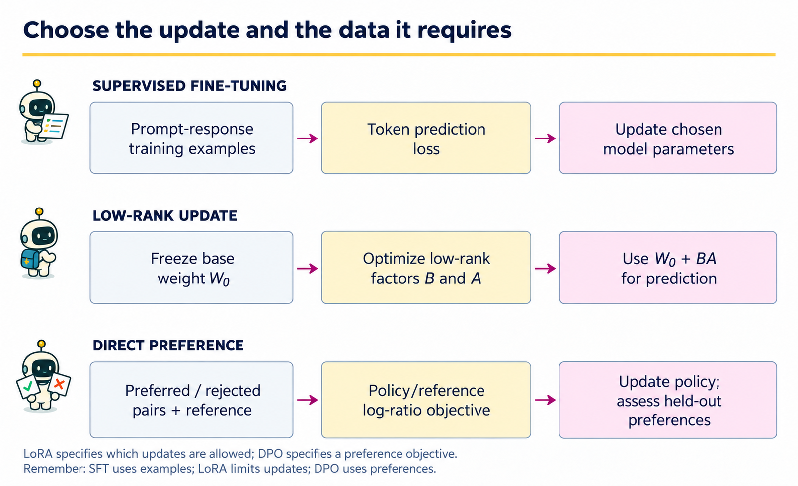
Separate the learning objective from the parameterization of the update. Supervised fine-tuning and preference optimization specify how examples are scored. LoRA specifies how weights are allowed to change. A model can therefore use LoRA while optimizing a supervised objective or a preference objective; the rows are not mutually exclusive product choices.
Decision |
Needed evidence |
Output and check |
|---|---|---|
Improve response behavior |
Desired prompt-response examples |
A supervised objective; check behavior on prompts excluded from fitting. |
Constrain adaptation cost |
A pretrained base and a chosen update rank |
Frozen base plus adapter weights; check the actual trainable parameter set. |
Learn preferences |
Comparable preferred/rejected responses for each prompt |
A preference objective and fixed reference; check held-out preference performance and task quality. |
Supply changing facts |
A maintained document collection |
Usually a retrieval intervention first; test whether the missing information is actually retrieved. |
The low-rank regression lab below isolates the geometric constraint. The discrete DPO lab isolates the preference objective. Neither is a full fine-tuning run on an LLM. When combining them in a larger system, save the base-model version, adapter configuration, reference-policy version, data split, and objective settings so that each intervention remains identifiable.
9.1 · Choose the intervention to match the problem#
Method |
What changes? |
A natural use |
|---|---|---|
Prompting |
Input context |
Specify a task or output convention |
Retrieval |
Evidence supplied in context |
Use a document collection that can be updated |
Supervised fine-tuning |
Model parameters |
Learn behavior from input/response examples |
LoRA |
Selected low-rank parameter updates |
Reduce the number of trainable parameters |
Preference optimization |
Parameters using comparisons |
Favor responses according to observed preferences |
Supervised fine-tuning minimizes a response-token negative log likelihood conditional on the instruction. Often the instruction tokens are excluded from that loss. Data provenance, duplicates, and separation by task or document matter: a large collection of nearly identical instructions is not equivalent to a large collection of independent tasks.
Define which tokens supervised tuning fits#
For instruction/response pairs \((x_i,y_i)\), write \(y_i=(y_{i1},\ldots,y_{iT_i})\), including any end marker used as a target. A token-weighted response-only objective is
The instruction is conditioning information; its tokens do not contribute targets in this convention. Padding is excluded too. A per-example mean would first divide each response loss by \(T_i\) and then average examples, changing the weighting. State the convention before comparing runs. LoRA below restricts which parameters can change; it can use Equation (9.1) in a language model, whereas our runnable example uses regression MSE.
9.2 · Low-rank adaptation as a constrained update#
Use row-vector inputs and a weight matrix \(W_0\in\mathbb R^{d_{in}\times d_{out}}\). We freeze \(W_0\) and fit
The update in Equation (9.2) has rank at most \(r\) and \(r(d_{in}+d_{out})\) trainable entries, compared with \(d_{in}d_{out}\) for a full update. The scale \(s\) is explicit; conventions often express it as a hyperparameter divided by rank. The restriction can reduce variance or prevent fitting a necessary high-rank change. It is not guaranteed to improve accuracy.
Initialize one factor randomly and the other at zero. If both factors start at zero, gradients of their product are zero and the update cannot begin learning.
Code
import numpy as np
import torch
from torch import nn
import matplotlib.pyplot as plt

torch.set_num_threads(1)
torch.manual_seed(9)
din, dout, rank = 12, 8, 2
W0 = torch.randn(din, dout) * 0.2
true_update = (torch.randn(din, rank) @ torch.randn(rank, dout)) * 0.15
X = torch.randn(250, din)
Y = X @ (W0 + true_update) + 0.1 * torch.randn(250, dout)
Xtr, Xte, Ytr, Yte = X[:50], X[50:], Y[:50], Y[50:]

def fit_update(low_rank):
    if low_rank:
        A = nn.Parameter(torch.randn(din, rank) * 0.03)
        B = nn.Parameter(torch.zeros(rank, dout))
        parameters = [A, B]
        update = lambda: A @ B
    else:
        delta = nn.Parameter(torch.zeros(din, dout))
        parameters = [delta]
        update = lambda: delta
    optimizer = torch.optim.Adam(parameters, lr=0.03)
    for _ in range(450):
        optimizer.zero_grad()
        loss = ((Xtr @ (W0 + update()) - Ytr)**2).mean()
        loss.backward()
        optimizer.step()
    with torch.no_grad():
        result = update().clone()
        train_mse = ((Xtr @ (W0+result)-Ytr)**2).mean().item()
        test_mse = ((Xte @ (W0+result)-Yte)**2).mean().item()
    return result, train_mse, test_mse

full, full_train, full_test = fit_update(False)
low, low_train, low_test = fit_update(True)
print('Trainable entries: full', din*dout, 'low-rank', rank*(din+dout))
print('Full update train/test MSE:', round(full_train, 4), round(full_test, 4))
print('Low-rank update train/test MSE:', round(low_train, 4), round(low_test, 4))
assert not W0.requires_grad
assert torch.linalg.matrix_rank(low, atol=1e-4) <= rank
Output
Trainable entries: full 96 low-rank 40
Full update train/test MSE: 0.0082 0.0135
Low-rank update train/test MSE: 0.0093 0.0117
The true update was deliberately chosen to have rank two. This favors the low-rank assumption and must be disclosed when interpreting results. To test robustness, replace it with a full-rank matrix, vary training size, and repeat the entire comparison. In transformers, low-rank updates may be attached to selected projection matrices; choosing their locations is another modeling decision.
Reconcile matrix conventions and initialization#
The diagram and the original LoRA paper use the common column-vector convention \(W_0+sBA\). Our code multiplies row inputs by a weight matrix on the right. Transposing the column convention gives
with \(A=A_{\mathrm{col}}^\top\in\mathbb R^{d_{\mathrm{in}}\times r}\) and \(B=B_{\mathrm{col}}^\top\in\mathbb R^{r\times d_{\mathrm{out}}}\). The factor names differ between conventions; the linear map does not. The scale \(s\) is fixed (one in this lab; often \(\alpha/r\) in LoRA).
For \(\Delta=sAB\) and \(G=\partial L/\partial\Delta\),
Equation (9.3) shows why, at \(B=0\) and random nonzero \(A\), the initial update is zero, but \(\nabla_B L\) can be nonzero. Once \(B\) moves, \(A\) can also receive a gradient. Initializing both factors at zero blocks both gradients. This explains the initialization choice without treating low rank as a different prediction objective.
Example 9.1 · A rank-one adapter cannot fit every update
Setup. In the row-vector convention of Equation (9.2), take \(d_{in}=3\), \(d_{out}=2\), \(r=1\), and \(s=1\). Let \(A=(1,2,0)^\top\) and \(B=(3,-1)\).
Work it through. The three rows of \(AB\) are \((3,-1)\), \((6,-2)\), and \((0,0)\). Every nonzero row is a multiple of the first, so the update has rank one. It trains \(3+2=5\) entries instead of 6 for a full update. A desired update with rows \((1,0)\), \((0,1)\), and \((0,0)\) has rank two and cannot be represented exactly by these rank-one factors.
What this shows. LoRA imposes a geometric restriction, not just a smaller file. Better optimization cannot remove that restriction. The tiny dimensions make the saving modest here; parameter savings and approximation quality are separate questions.
9.3 · Inspect the fitted update, not only parameter counts#
Code
fig, ax = plt.subplots(figsize=(5, 3.2))
for name, matrix, color in [('True', true_update, '#705600'),
                             ('Full fit', full, '#777777'),
                             ('Low-rank fit', low, '#a2006e')]:
    singular = torch.linalg.svdvals(matrix).numpy()
    ax.plot(range(1, len(singular)+1), singular, 'o-', label=name, color=color)
ax.set(xlabel='Singular-value index', ylabel='Singular value')
ax.legend()
plt.tight_layout()
plt.show()
Output
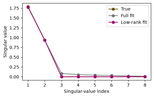
A low-rank parameterization is a restriction on an update in parameter space, not a claim that all task information is low-dimensional. Parameter count alone also does not determine training memory: activations, optimizer state, precision, and frozen-weight storage still matter.
9.4 · Preference observations and Bradley–Terry probabilities#
For a prompt \(x\), suppose a latent utility function \(r(x,y)\) determines pairwise preference probabilities:
Adding a constant to all utilities for a prompt leaves these probabilities unchanged. The model describes a population of preference observations, not an objective notion of truth. Annotator selection, ambiguous instructions, response length, presentation order, and disagreement all affect the labels.
A common RLHF formulation fits a reward model from comparisons and then optimizes expected reward while penalizing KL divergence from a reference policy. For a fixed prompt and unrestricted policy, maximizing \(\mathbb E_\pi r-\beta\operatorname{KL}(\pi\Vert\pi_{ref})\) yields \(\pi^*(y)\propto\pi_{ref}(y)e^{r(y)/\beta}\), assuming the relevant support and normalizer conditions.
From a KL penalty to a policy ratio#
For fixed prompt \(x\) and \(\beta>0\), suppose \(\pi_{\mathrm{ref}}\) has support on every allowed response and the following sum is finite:
Rearranging Equation (9.5) yields
The prompt-specific constant cancels when comparing two responses. Substituting a trainable \(\pi_\theta\) for \(\pi^*\) produces the paired logistic objective below, following DPO. Here \(\beta\) controls the reference penalty, not the sampling temperature. The closed-form optimum assumes unrestricted policies; a finite neural family and noisy optimization need not attain it.
9.5 · A tiny direct-preference objective#
Substituting the reward representation in Equation (9.6) into the Bradley–Terry model in Equation (9.4), then replacing \(\pi^*\) by \(\pi_\theta\), gives the DPO loss for a preferred response \(y_w\) and a dispreferred response \(y_l\):
The code optimizes Equation (9.7) using one prompt with three possible responses, a uniform reference, and simulated noisy preferences. For language models, each response log probability is a sum of token log probabilities, with careful handling of prompt masking and sequence length. The discrete example makes the reference term and preference direction easy to verify.
Code
rng = np.random.default_rng(90)
utilities = np.array([1.2, 0.3, -0.8])
pairs = np.array([rng.choice(3, size=2, replace=False) for _ in range(500)])
p_first = 1 / (1 + np.exp(-(utilities[pairs[:, 0]]-utilities[pairs[:, 1]])))
first_wins = rng.random(len(pairs)) < p_first
winners = torch.tensor(np.where(first_wins, pairs[:, 0], pairs[:, 1]))
losers = torch.tensor(np.where(first_wins, pairs[:, 1], pairs[:, 0]))
train_ids, test_ids = np.arange(400), np.arange(400, 500)
reference = torch.full((3,), 1/3)
policy_logits = nn.Parameter(torch.zeros(3))
optimizer = torch.optim.Adam([policy_logits], lr=0.03)
beta_preference = 0.7
for _ in range(300):
    optimizer.zero_grad()
    log_ratio = torch.log_softmax(policy_logits, dim=0) - reference.log()
    margin = beta_preference * (log_ratio[winners[train_ids]]-log_ratio[losers[train_ids]])
    loss = -nn.functional.logsigmoid(margin).mean()
    loss.backward()
    optimizer.step()
with torch.no_grad():
    policy = torch.softmax(policy_logits, dim=0)
    ratio = policy.log()-reference.log()
    test_margin = beta_preference*(ratio[winners[test_ids]]-ratio[losers[test_ids]])
    heldout_loss = -nn.functional.logsigmoid(test_margin).mean().item()
print('Reference probabilities:', reference.numpy().round(3))
print('Fitted probabilities:', policy.numpy().round(3))
print('Held-out preference log loss:', round(heldout_loss, 3))
print('Equal-preference log loss:', round(np.log(2), 3))
Output
Reference probabilities: [0.333 0.333 0.333]
Fitted probabilities: [0.72  0.216 0.063]
Held-out preference log loss: 0.486
Equal-preference log loss: 0.693
This test holds out comparison draws, not new prompts. It evaluates the same three-response preference problem under additional label noise. It cannot establish generalization to new tasks or factual correctness. The reference policy has positive probability on every response, so its log ratios are defined.
Example 9.2 · DPO compares changes relative to a reference
Setup. There are two possible responses, preferred \(y_w\) and rejected \(y_l\). Let the reference probabilities be \((0.8,0.2)\), the current policy be \((0.6,0.4)\), and \(\beta=1\).
Work it through. The margin in Equation (9.7) is \(\log(0.6/0.8)-\log(0.4/0.2)=\log(0.375)\approx-0.9808\). Its logistic probability is \(0.375/(1+0.375)=3/11\approx0.2727\), giving loss \(-\log(3/11)\approx1.2993\). If policy and reference agreed, the margin would be zero and the loss would be \(\log2\approx0.6931\).
What this shows. The current policy still assigns more absolute probability to the preferred response, yet it favors that response less strongly than the reference did. DPO evaluates this relative shift. Its pairwise probability is part of a preference model, not a factual-correctness probability for either response.
9.6 · Design an adaptation evaluation#
Keep separate evaluations for task quality, instruction compliance, factual support, and resource cost. Use a baseline with the same retrieval access and decoding budget. If preference tuning improves a judge score, inspect whether response length or style changed in a way the judge rewards independently of correctness.
Record the base model, adaptation data, frozen parameters, trainable parameters, optimizer, checkpoint rule, and evaluation split. Prevent task-family leakage where paraphrases of the same underlying question appear in both training and testing. A comparison against an untuned baseline is informative only if the baseline receives an appropriate prompt and comparable evidence.
Coding and experiment practice · Compare low-rank and full updates#
1. Predict before running. For input width 12, output width 8 and rank 2, how many trainable entries are there? Does rank two constrain the full adapted weight?
2. Implement and check. Check rank and parameter count, then refit the low-rank and full update on identical data with 450 optimizer steps each. Keep rank choice separate from final test reporting. The code below is a worked example. For independent work, download Assignment 09, which has an empty implementation, separate acceptance fixtures and a new transfer task. Attempt it before opening the separate solution file.
Code
def lora_parameter_count(d_in, d_out, update_rank):
    return update_rank * (d_in + d_out)

assert lora_parameter_count(12, 8, 2) == 40
assert lora_parameter_count(3, 5, 1) == 8
assert lora_parameter_count(3, 5, 2) == 16
fixture_A = torch.tensor([[1.], [2.], [3.]])
fixture_B = torch.tensor([[1., -1.]])
assert torch.linalg.matrix_rank(fixture_A @ fixture_B, atol=1e-6) == 1
comparison_rows = []
for seed in [91, 92, 93]:
    for constrained in [False, True]:
        torch.manual_seed(seed)
        delta, train_error, test_error = fit_update(constrained)
        count = lora_parameter_count(din, dout, rank) if constrained else din*dout
        comparison_rows.append((seed, constrained, count, train_error, test_error))
        if constrained:
            assert torch.linalg.matrix_rank(delta, atol=1e-4) <= rank
print('Seed / low rank / parameters / train MSE / test MSE')
for row in comparison_rows:
    print(row)
Output
Seed / low rank / parameters / train MSE / test MSE
(91, False, 96, 0.008189053274691105, 0.013526544906198978)
(91, True, 40, 0.009340641088783741, 0.011721049435436726)
(92, False, 96, 0.008189053274691105, 0.013526544906198978)
(92, True, 40, 0.009340641088783741, 0.011721049435436726)
(93, False, 96, 0.008189053274691105, 0.013526544906198978)
(93, True, 40, 0.00934097170829773, 0.011730912141501904)
fit_update uses the fixed training and test arrays defined above, creates a fresh optimizer, and performs the same declared number of steps. The seeds vary initialization, not training datasets; these repetitions cannot measure dataset-sampling uncertainty. The rank restriction applies to the update, not W0 + update.
3. Extend one factor. On a new development experiment change the generating update from rank two to full rank. Keep data size, noise and optimization budgets fixed. Declare which setting favors the structural assumption. This numerical experiment is a bridge to LoRA, not a claim that a pretrained LLM was fine-tuned.
Submission and rubric. Submit the function and its checks, the requested comparison table, and three sentences naming the target, interpreting the result, and limiting the claim. Passing a deterministic fixture verifies the stated calculation; a favorable stochastic result is not required. Retain unexpected results and diagnose them rather than changing seeds until a preferred ranking appears.
9.7 · Exercises#
Parameter budget: for a \(1024\times1024\) update with rank eight, how many entries are trained?
Initialization: derive \(\nabla_A L\) and \(\nabla_B L\) when \(\Delta=AB\).
Identifiability: does paired-comparison data identify an absolute utility level?
DPO direction: if policy and reference initially agree, what is each margin?
Scope: why might a rank-two update fail even with excellent optimization?
Worked solutions — attempt the questions first
1. \(8(1024+1024)=16,384\), versus \(1,048,576\) for a full update. This counts update parameters, not the entire model’s stored weights.
2. if \(G=\nabla_\Delta L\), the gradients are \(GB^\top\) and \(A^\top G\). Both vanish if both factors are zero.
3. no. It identifies differences under the model, since adding a common constant leaves all comparison probabilities unchanged.
4. zero. The loss is \(\log2\). Updating increases the preferred response’s log ratio relative to the dispreferred response, subject to shared parameters and conflicting observations.
5. the necessary parameter change may have higher rank or may be needed in layers that were not adapted. More optimization cannot remove a restriction imposed by the model class.
9.8 · Reading and transition#
LoRA develops low-rank parameter updates for large models. DPO connects preference likelihoods with a reference-policy formulation. Next, Chapter 10 changes the evidence available at inference time while leaving model weights fixed.