11 · Evaluation, calibration, and uncertainty

Question. What evidence would justify saying one system is better than another?

Download the executed notebook

Python support: Read A.9: JSON and validation and A.11: local modules and kernels before the implementation. Use Show all code while working.

An evaluation begins with a target population and a loss, not with a leaderboard. We will compare paired system outcomes, estimate uncertainty by resampling questions, examine calibration and abstention, and construct finite-label conformal prediction sets. All numerical outcomes in this chapter are simulated; they illustrate statistical procedures rather than measure any commercial or pretrained model.

Prerequisites: Chapters 1, 6, and 10; sampling distributions and quantiles. Outcomes: define an estimand; preserve pairing; separate calibration from discrimination; interpret risk–coverage curves; state a conformal guarantee precisely.

Pipeline and framework

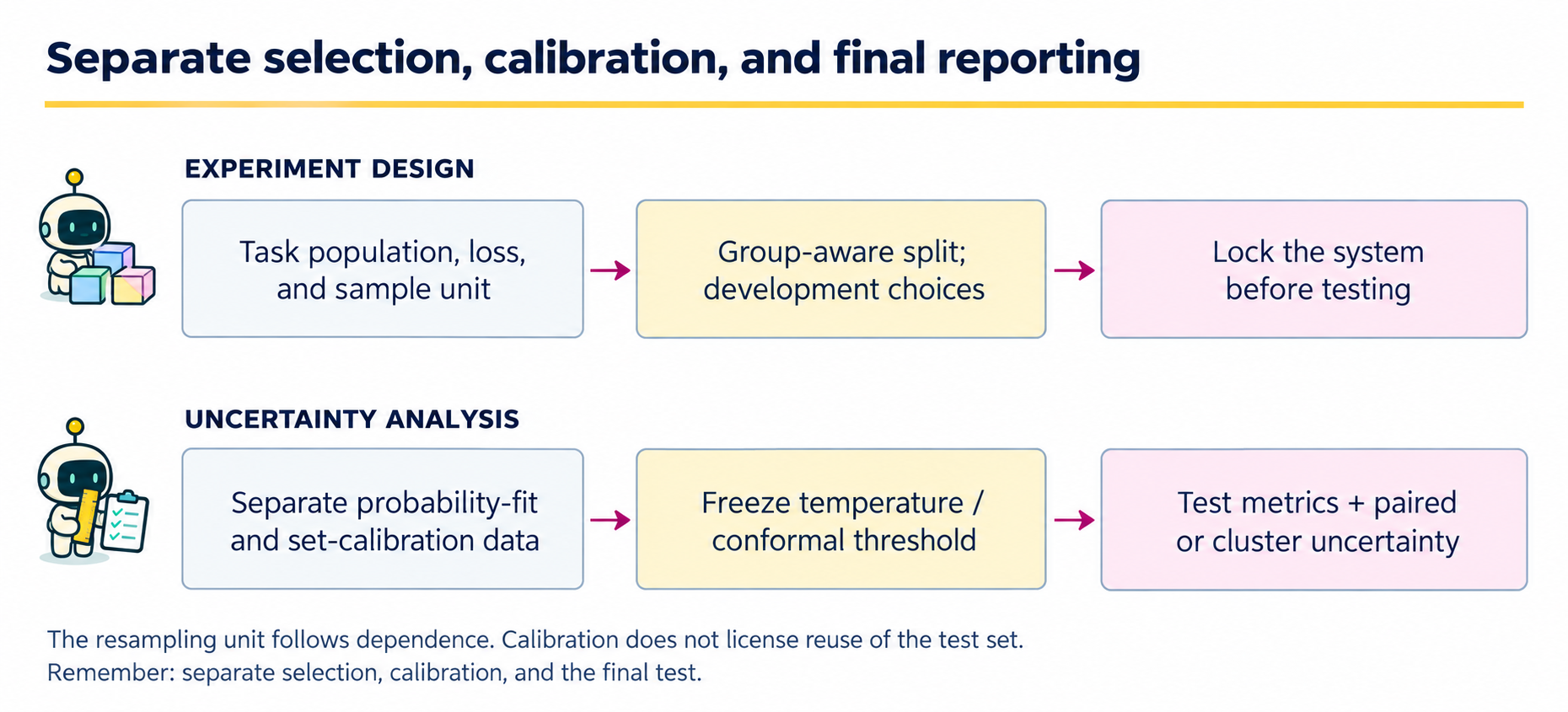
Evaluation is a data-use protocol, not a final call to a metric function. Write down which sample is allowed to influence each choice before fitting anything. In the executable classifier example, temperature is fitted on a validation sample, the conformal threshold is computed on a different calibration sample, and both are evaluated on a test sample.

Data or artifact	Permitted role	Prohibited shortcut
Development data	Choose prompts, architectures, retrieval settings, and stopping rules.	Repeatedly choosing settings on the final test outcomes.
Probability-fitting data	Fit a calibration map such as temperature scaling.	Claiming out-of-sample calibration from fitted-sample reliability alone.
Conformal calibration data	Compute a quantile after the score function is fixed.	Reusing those labels to tune the same score function without an appropriate method.
Final test data	Estimate locked-system performance and uncertainty.	Treating multiple calls on one task as independent sampled tasks.

The framework has two outputs: a performance estimate and an account of what it generalizes to. For a system comparison, pair outputs on the same questions. For repeated agent trials, preserve the task cluster. For conformal sets, state the marginal guarantee and exchangeability requirement rather than reading the guarantee as certainty for every subgroup or individual question.

11.1 · Define the estimand and the unit

Let \(Q\) be a question drawn from the intended task population and \(U\) represent generation randomness. A system’s risk is \(R=\mathbb E[\ell(f(Q,U),Y)]\). A comparison might target \(R_B-R_A\) under a fixed model version, prompt, retrieval collection, and decoding budget. Changing any of these changes the procedure under evaluation.

The sampling unit is usually the question, user, document, or task family, not each token and not necessarily each generation. Repeated answers to the same question share difficulty and evidence. If questions share documents, resample documents or use another method appropriate to that dependence.

11.2 · Preserve pairing when comparing systems

Code

import numpy as np
import matplotlib.pyplot as plt

rng = np.random.default_rng(11)
n = 240
difficulty = rng.normal(size=n)
p_a = 1/(1+np.exp(-(0.6-difficulty)))
p_b = 1/(1+np.exp(-(0.85-difficulty)))
# Shared task difficulty induces pairing; independent residual draws allow gains and losses.
correct_a = rng.random(n) < p_a
correct_b = rng.random(n) < p_b
difference = correct_b.astype(float)-correct_a.astype(float)
bootstrap_ids = rng.integers(n, size=(3000, n))
bootstrap_difference = difference[bootstrap_ids].mean(1)
interval = np.quantile(bootstrap_difference, [0.025, 0.975])
print('A-only / B-only successes:', int((correct_a & ~correct_b).sum()),
      int((correct_b & ~correct_a).sum()))
print('Accuracy A / B:', correct_a.mean().round(3), correct_b.mean().round(3))
print('Paired accuracy difference B-A:', round(difference.mean(), 3))
print('Question-bootstrap percentile interval:', interval.round(3))

Output

A-only / B-only successes: 45 51
Accuracy A / B: 0.638 0.662
Paired accuracy difference B-A: 0.025
Question-bootstrap percentile interval: [-0.054  0.104]

The shared task difficulty induces association, while separate conditional draws allow both A-only and B-only successes. This is a simulation design, not a claim about actual LLM error dependence. Resampling the paired differences preserves the observed association between systems. Resampling A and B independently would estimate a different sampling variance.

A percentile bootstrap interval is an approximation, not an exact finite-sample guarantee. Its interpretation depends on the sampled tasks representing the target population. It does not account for an unreported search over prompts or models using the same test set.

Why pairing changes uncertainty

For independent sampled questions, let \(A_i,B_i\in\{0,1\}\) indicate correctness and \(D_i=B_i-A_i\). The accuracy estimand and estimator are

(11.1)\[ \Delta=\mathbb E[D_i],\qquad \widehat\Delta=\frac1n\sum_iD_i,\qquad \widehat{\operatorname{SE}}(\widehat\Delta)=\frac{s_D}{\sqrt n}, \]

where \(s_D^2=(n-1)^{-1}\sum_i(D_i-\widehat\Delta)^2\). The population identity

\[ \operatorname{Var}(D_i)=\operatorname{Var}(B_i)+\operatorname{Var}(A_i) -2\operatorname{Cov}(A_i,B_i) \]

explains why independently resampling the two systems loses information. The code resamples whole paired differences to estimate uncertainty in Equation (11.1), using bootstrap quantiles rather than its normal-approximation standard error. For zero-one loss, the risk difference \(R_B-R_A=-\Delta\); report the direction so a positive improvement is not mistaken for a larger loss.

Example 11.1 · Paired outcomes reveal which questions changed

Setup. On five shared questions, system A has correctness indicators \((1,1,0,0,1)\) and B has \((1,0,1,0,1)\).

Work it through. Both accuracies are \(3/5\), so the estimated improvement is zero. The paired differences are \((0,-1,1,0,0)\): B loses one question and gains another. Their sample variance is \((1+1)/(5-1)=0.5\), giving estimated standard error \(\sqrt{0.5/5}\approx0.3162\) in Equation (11.1). A bootstrap draw must resample these whole question-level differences, retaining each A/B pair.

What this shows. Equal aggregate accuracy does not mean identical behavior or a precisely known population difference. The paired record preserves where outcomes changed. Five questions are too few for a persuasive performance claim; they make the accounting easy to inspect.

11.3 · Separate factual labels from judging machinery

For open-ended answers, define a rubric before viewing system identities: factual support, completeness, relevance, and required abstention may need separate labels. Use blinded ordering and audit disagreements. An LLM judge is another measurement instrument, with potential style preferences, positional effects, and shared errors with the evaluated system.

Report how labels were obtained and whether repeated annotations are independent. A high judge score is not automatically factual correctness. When feasible, include exact-answer checks or evidence-grounded human adjudication for a subset and quantify disagreement rather than silently resolving it in favor of one system.

11.4 · Calibration is a relationship between probabilities and outcomes

For binary outcomes, calibration informally asks whether events assigned probability \(p\) occur at frequency \(p\). A model can rank cases well while being overconfident. The Brier score averages \((p-y)^2\); log loss strongly penalizes confidently wrong probabilities. A binned reliability plot is descriptive and depends on bin definitions and sample size.

Calibration and temperature scaling in symbols

For a binary probability prediction \(P\in[0,1]\), population calibration means

(11.2)\[ \mathbb E[Y\mid P]=P\quad\text{almost surely}. \]

It does not require a continuous predictor to take any exact prespecified value with positive probability. Bins estimate averages of this relationship. On \(n\) evaluation cases, the Brier score is \(n^{-1}\sum_i(p_i-y_i)^2\); it measures overall probability error, not calibration alone.

For fixed logits \(z_i\), temperature fitting on the separate validation index set \(\mathcal V\) is

(11.3)\[ \widehat\tau\in\operatorname*{arg\min}_{\tau\in\mathcal T} \frac1{|\mathcal V|}\sum_{i\in\mathcal V} \left[\log(1+e^{z_i/\tau})-y_i z_i/\tau\right], \qquad \widetilde p_i=\sigma(z_i/\widehat\tau). \]

\(\mathcal T\subset(0,\infty)\) is the finite grid used below. logaddexp evaluates the first term stably. Positive temperature preserves binary ranking and the zero-logit decision boundary; it can improve probabilities without changing 0.5-threshold accuracy. Fitting Equation (11.3) does not guarantee the population calibration property in Equation (11.2).

Below a fixed simulated predictor is deliberately overconfident. A temperature is selected using a validation sample. We then evaluate on a disjoint test sample; a separate calibration sample is reserved for conformal prediction.

Code

n_total = 1400
latent = rng.normal(size=n_total)
true_p = 1/(1+np.exp(-latent))
y = rng.binomial(1, true_p)
logits = 2.0 * latent
validation = np.arange(300)
calibration = np.arange(300, 800)
test = np.arange(800, n_total)

def sigmoid(z):
    return 1/(1+np.exp(-z))

def binary_loss(z, labels):
    return np.mean(np.logaddexp(0, z)-labels*z)

temperatures = np.linspace(0.5, 3.5, 121)
validation_losses = [binary_loss(logits[validation]/t, y[validation]) for t in temperatures]
temperature = temperatures[np.argmin(validation_losses)]
raw_p = sigmoid(logits[test])
calibrated_p = sigmoid(logits[test]/temperature)
print('Validation-selected temperature:', round(temperature, 3))
for label, p in [('Raw', raw_p), ('Temperature-scaled', calibrated_p)]:
    print(label, 'Brier:', round(np.mean((p-y[test])**2), 3))

fig, ax = plt.subplots(figsize=(4.5, 3.7))
for label, p, color in [('Raw', raw_p, '#705600'),
                       ('Scaled', calibrated_p, '#a2006e')]:
    bins = np.minimum((p*8).astype(int), 7)
    points = [(p[bins==b].mean(), y[test][bins==b].mean())
              for b in range(8) if np.sum(bins==b) >= 10]
    ax.plot(*np.array(points).T, 'o-', label=label, color=color)
ax.plot([0, 1], [0, 1], ':', color='gray')
ax.set(xlabel='Mean predicted probability', ylabel='Observed event fraction',
       xlim=(0, 1), ylim=(0, 1))
ax.legend()
plt.tight_layout()
plt.show()

Output

Validation-selected temperature: 1.75
Raw Brier: 0.213
Temperature-scaled Brier: 0.202

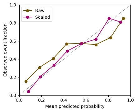
Temperature scaling preserves the ranking of binary logits when temperature is positive. It changes probability calibration, not the underlying evidence. Token probabilities from a language model are probabilities of token events under that model; they are not automatically probabilities that a whole answer is factually correct.

11.5 · Abstention produces a risk–coverage tradeoff

Let \(c_i\) be a confidence score and answer only if \(c_i\ge\tau\). Coverage is the answered fraction. Selective risk is the average loss among answered cases. Both quantities matter.

For \(A_\tau=\mathbf1\{c(Q)\ge\tau\}\) and a fixed system loss \(L\), the population quantities are

(11.4)\[ \operatorname{Coverage}(\tau)=\mathbb P(A_\tau=1),\qquad \operatorname{Risk}(\tau)=\frac{\mathbb E[L A_\tau]}{\mathbb E[A_\tau]}. \]

The empirical counterparts of Equation (11.4) are \(n^{-1}\sum_i A_{\tau i}\) and \(\sum_i\ell_i A_{\tau i}/\sum_i A_{\tau i}\). Selective risk is defined only at positive coverage. In this lab \(c_i=\max(\widetilde p_i,1-\widetilde p_i)\) and \(\ell_i\) is a binary classification error. These definitions also apply to answer/abstain decisions in RAG after defining a suitable answer-level loss and confidence score.

Code

confidence = np.maximum(calibrated_p, 1-calibrated_p)
prediction = calibrated_p >= 0.5
errors = (prediction != y[test]).astype(float)
thresholds = np.linspace(0.5, 0.9, 30)
coverage, risk = [], []
for threshold in thresholds:
    selected = confidence >= threshold
    if selected.any():
        coverage.append(selected.mean())
        risk.append(errors[selected].mean())
fig, ax = plt.subplots(figsize=(5, 3.3))
ax.plot(coverage, risk, 'o-', markersize=3, color='#a2006e')
ax.set(xlabel='Coverage: fraction answered', ylabel='Error among answered cases',
       title='Descriptive test risk–coverage curve')
plt.tight_layout()
plt.show()

Output

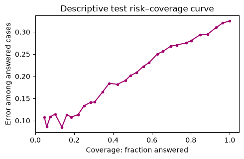
This curve is descriptive. If you use it to choose the operating threshold, this test sample has become development data. For a final evaluation, choose the threshold on a separate development set and report uncertainty on a new test set. Risk can also worsen within an important subgroup even when overall selective risk improves.

Example 11.2 · A lower error rate can hide fewer answers

Setup. On 100 held-out questions, a system answers all questions and gets 20 wrong. A threshold fixed on separate development data keeps 60 answers, of which 3 are wrong.

Work it through. Before filtering, coverage is 1 and risk is \(20/100=0.20\). After filtering, Equation (11.4) gives coverage \(60/100=0.60\) and selective risk \(3/60=0.05\). The retained correct answers number 57, while the original system had 80 correct answers overall.

What this shows. “95% correct when answering” describes a different service level from “answers every question.” Report both quantities, plus subgroup behavior where relevant. If the threshold retained no answers, coverage would be zero and selective risk would be undefined, rather than evidence of a perfect system.

11.6 · Split conformal prediction for a finite label space

We now construct sets of labels in \(\{0,1\}\) using a predictor fixed before the conformal calibration sample is examined. For calibration case \(i\), use nonconformity score \(s_i=1-\widehat p_{y_i}(x_i)\). With \(n_c\) calibration cases, let \(k=\lceil(n_c+1)(1-\alpha)\rceil\) and take the kth smallest score. If \(k>n_c\), use an infinite threshold. The set is

(11.5)\[ C(x)=\{y:1-\widehat p_y(x)\le \widehat q\}. \]

Under exchangeability of calibration and future examples, with the predictor fixed independently of these calibration outcomes, this construction gives marginal coverage at least \(1-\alpha\). Ties make the nonrandomized version potentially conservative. The guarantee is over calibration and future examples jointly, not a guarantee of coverage conditional on every covariate value.

In symbols, with \(s_{(k)}\) the kth ordered calibration score,

(11.6)\[\begin{split} \widehat q=\begin{cases}s_{(k)},&k\le n_c,\\+\infty,&k=n_c+1,\end{cases} \quad k=\lceil(n_c+1)(1-\alpha)\rceil,\quad 0<\alpha<1, \end{split}\]

(11.7)\[ \mathbb P_{\mathcal D_{\mathrm{cal}},(X_{\mathrm{new}},Y_{\mathrm{new}})} \{Y_{\mathrm{new}}\in C(X_{\mathrm{new}})\}\ge 1-\alpha. \]

Equation (11.7) applies to the set in Equation (11.5) with the threshold in Equation (11.6). For distinct exchangeable scores, the new score’s rank among \(n_c+1\) scores is uniform; choosing this rank gives the finite-sample correction. Ties with the displayed non-strict inclusion preserve the lower bound. The probability averages over both a new calibration sample and a future case, conditional on the independently fitted predictor; it is not a statement that every realized calibration sample or every covariate subgroup has coverage \(1-\alpha\). See the split-conformal construction.

Code

alpha = 0.1
p_cal = sigmoid(logits[calibration]/temperature)
P_cal = np.column_stack([1-p_cal, p_cal])
scores = 1-P_cal[np.arange(len(calibration)), y[calibration]]
k = int(np.ceil((len(scores)+1)*(1-alpha)))
q = np.sort(scores)[k-1] if k <= len(scores) else np.inf
P_test = np.column_stack([1-calibrated_p, calibrated_p])
sets = (1-P_test) <= q
covered = sets[np.arange(len(test)), y[test]]
print('Calibration size / rank / quantile:', len(scores), k, round(q, 3))
print('Empirical test coverage:', round(covered.mean(), 3))
print('Average set size:', round(sets.sum(1).mean(), 3))
print('Empty / singleton / doubleton counts:', np.bincount(sets.sum(1), minlength=3))

Output

Calibration size / rank / quantile: 500 451 0.692
Empirical test coverage: 0.898
Average set size: 1.505
Empty / singleton / doubleton counts: [  0 297 303]

The observed test fraction can lie below the nominal level in one finite sample. Equation (11.7) does not assert that every test batch achieves the target exactly. Larger prediction sets may deliver coverage while being less informative. Evaluate both coverage and set size.

A set of finite class labels is not a set of all semantically correct free-text answers. Applying conformal ideas to generated text requires specifying an assessable target, a score, and assumptions appropriate to that target. Distribution shift, adaptive reuse of calibration data, and dependence can invalidate a naive guarantee.

Example 11.3 · A conformal threshold produces a set

Setup. With a fixed predictor, suppose nine calibration scores are \(0.05,0.10,0.15,0.20,0.25,0.30,0.40,0.60,0.80\). Choose \(\alpha=0.2\).

Work it through. Equation (11.6) uses rank \(\lceil(9+1)(0.8)\rceil=8\), so \(\widehat q=0.60\). A new binary prediction \((p_0,p_1)=(0.7,0.3)\) has label scores \((0.3,0.7)\); Equation (11.5) retains only label 0. Prediction \((0.5,0.5)\) has scores \((0.5,0.5)\), so it retains both labels.

What this shows. The threshold is shared, but the prediction-set size depends on the case. Under the stated exchangeability and fixed-predictor assumptions, the guarantee concerns marginal coverage across calibration samples and future cases. It does not assign an 80% correctness probability to either of these particular sets.

Pair the actual Chapter 10 rows before interpreting uncertainty

This uses the same saved RAG responses and reviews as Chapter 10. Joining on task identity protects the observational unit when rows are reordered. A missing condition or unreviewed success label is an error, not a row to drop.

Code

from pathlib import Path
import os
import sys

start = Path(os.environ.get('GENAI_COURSE_ROOT', Path.cwd())).resolve()
root = None
# Examine this folder, then each enclosing folder.
candidates = [start] + list(start.parents)
for candidate in candidates:
    if (candidate / 'labs/model.json').is_file():
        root = candidate
        break
if root is None:
    raise FileNotFoundError('Keep the notebook inside Teaching-GenAI, or set GENAI_COURSE_ROOT')
if str(root) not in sys.path:
    sys.path.insert(0, str(root))
from labs.evaluation import load_evaluation, paired_scores, make_row, validate_rows
common_rows = load_evaluation(root)
rag_rows = []
for row in common_rows:
    if row['task_family'] == 'rag':
        rag_rows.append(row)
rag_pairs = paired_scores(rag_rows, 'extractive', 'llm')
print('Descriptive paired task rows:', rag_pairs)
assert len(rag_pairs) == 1

Output

Descriptive paired task rows: [{'task_id': 'dependent-bootstrap', 'replicate': 0, 'a': 1.0, 'b': 1.0, 'difference': 0.0}]

There is only one authored RAG question here. Its observed contrast is a descriptive check, not an estimate supported by a sampled task population. The 240-task simulation earlier in the chapter teaches interval mechanics under its explicit sampling model; it must not be presented as 240 actual model evaluations. Repeated trajectories stay within the same task cluster.

Coding and experiment practice · Preserve pairing and numeric meaning

1. Predict before running. For A=[True, False, True] and B=[False, True, True], what signed differences represent losses and gains?

2. Implement and check. Convert Boolean scores to floating-point numbers before subtraction. Validate paired, nonempty one-dimensional inputs, then return a vector of bootstrap mean differences. The code below is a worked example. For independent work, download Assignment 11, which has an empty implementation, separate acceptance fixtures and a new transfer task. Attempt it before opening the separate solution file.

Code

def paired_bootstrap(a, b, seed=11, draws=2000):
    a, b = np.asarray(a, dtype=float), np.asarray(b, dtype=float)
    if a.ndim != 1 or a.shape != b.shape or len(a) == 0:
        raise ValueError('Use nonempty paired one-dimensional score vectors')
    if not np.isfinite(a).all() or not np.isfinite(b).all():
        raise ValueError('Scores must be finite')
    difference = b - a
    rng = np.random.default_rng(seed)
    indices = rng.integers(len(a), size=(draws, len(a)))
    return difference[indices].mean(axis=1)

fixture_a = np.array([True, False, True])
fixture_b = np.array([False, True, True])
assert np.array_equal(fixture_b.astype(float)-fixture_a.astype(float), [-1., 1., 0.])
assert np.all(paired_bootstrap(fixture_a, fixture_a) == 0)
assert np.all(paired_bootstrap([False], [True]) == 1)
assert np.all(paired_bootstrap([True], [False]) == -1)
bootstrap_fixture = paired_bootstrap(fixture_a, fixture_b)
assert bootstrap_fixture.shape == (2000,)
assert np.isfinite(bootstrap_fixture).all()
print('Signed paired differences:', fixture_b.astype(float)-fixture_a.astype(float))
print('Fixture bootstrap range:', bootstrap_fixture.min(), bootstrap_fixture.max())

Output

Signed paired differences: [-1.  1.  0.]
Fixture bootstrap range: -1.0 1.0

NumPy does not support Boolean subtraction; exclusive-or would erase the sign and therefore answer the wrong question. Each sampled index retains a whole A/B pair. The three-case fixture verifies mechanics only; it does not justify a useful population confidence interval.

3. Extend one factor. Apply the function to the chapter synthetic experiment containing gains and losses. For real outputs, first specify the task population and sampling unit. The few authored live-lab cases support descriptive comparisons, not population intervals. Repeated generations of one question remain one task cluster.

Submission and rubric. Submit the function and its checks, the requested comparison table, and three sentences naming the target, interpreting the result, and limiting the claim. Passing a deterministic fixture verifies the stated calculation; a favorable stochastic result is not required. Retain unexpected results and diagnose them rather than changing seeds until a preferred ranking appears.

Continue with the implemented system

Appendix B supplies actual model outputs for a measurement audit. Its tiny authored task set supports descriptive counts, not a reliable population confidence interval. Use its keyword and schema checks as examples of measurement instruments that can disagree; inspect semantic support separately.

11.7 · Exercises

1. Paired estimator: write the estimand for the accuracy difference.

2. Repeated generations: why are 20 answers to each of 10 questions not 200 independent questions?

3. Conformal rank: with \(n_c=99\) and \(\alpha=0.1\), which order statistic is used?

4. Calibration leakage: can temperature be chosen using the same outcomes later used for an ordinary split-conformal quantile?

5. No answers: what is selective risk when no cases are answered?

6. Scope of coverage: does 90% marginal coverage imply 90% coverage for each subgroup?

Worked solutions — attempt the questions first

1. \(\mathbb E[1\{B\text{ correct}\}-1\{A\text{ correct}\}]\) on the target task distribution. The sample mean of question-level differences estimates it under representative sampling.

2. repetitions share a task. They help estimate within-question generation variability but provide only 10 question clusters for variation across tasks.

3. \(\lceil100(0.9)\rceil=90\). The finite-sample correction uses \(n_c+1\), not simply an interpolated 90th percentile.

4. that violates the simple fixed-predictor calibration argument. Use a separate fitting/validation sample or a method whose proof accounts for that data reuse.

5. it is undefined because its denominator is zero. Report zero coverage and an undefined risk, not a perfect zero error rate.

6. no. Marginal guarantees average across the target distribution. Group-specific guarantees require additional design and assumptions.

11.8 · Reading and next step

A Gentle Introduction to Conformal Prediction provides the formal framework and extensions behind the finite-label exercise. Next, Chapter 12 adds sequential tool decisions, which introduces new units of evaluation and additional failure modes.