3. Learning from positives and unlabelled observations#
Topics of Statistical Learning · Week 3
What is missing?#
In positive–unlabelled learning, some observations are known to belong to a positive class, while an unlabelled collection contains both classes. Examples include confirmed relevant documents and a broader document collection, or confirmed examples of a phenomenon together with background observations. An unlabelled observation has an unknown class, not a known negative class.
The main task is to express a target classification risk using distributions from which data are actually available. The derivation is short, but its sampling assumptions are consequential. We first use an explicit two-sample model, then distinguish it from a single dataset in which only some positive labels are revealed.
The two-sample model#
Let \(Y\in\{+1,-1\}\), let \(\pi=P(Y=+1)\in(0,1)\) be the target class prior, and write
The target feature marginal is
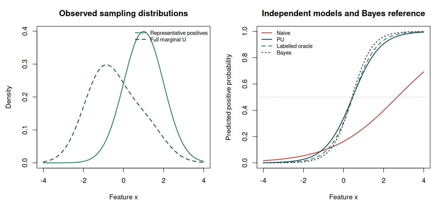
The introductory sampling scheme provides independent observations \(X^+_1,\ldots,X^+_{n_+}\sim P_+\) and \(X^U_1,\ldots,X^U_{n_U}\sim P_U\). These are representative samples from the specified positive distribution and the full target feature marginal. For now, \(\pi\) is known.
The ratio \(n_+/(n_++n_U)\) is controlled by data collection and is not an estimator of the target prevalence in this two-sample design. We may deliberately collect many confirmed positives while the target population contains relatively few positives.
Deriving the PU risk identity#
For a score \(g\) and loss \(\ell\), define \(\ell_\pm(X)=\ell(g(X),\pm1)\). The ordinary population risk is
The unavailable negative expectation can be removed by applying the mixture relation to \(\ell_-\):
Substituting gives
Each expectation on the right can be estimated from the observed samples. The subtraction removes the positive-class contribution that would otherwise be counted when unlabelled observations are temporarily evaluated as negative.
The identity applies to a loss with finite relevant expectations. It is not restricted to zero–one loss. Its empirical version is
For a fixed \(g\) and the stated known-prior sampling model, this estimator is unbiased. A model fitted by minimizing it still needs generalization analysis or independent evaluation. The fitted model is not fixed with respect to its training sample.
Worked example 3.1 — Removing positive contamination
Suppose \(\pi=0.3\), sensitivity is \(0.8\), and the false-positive rate is \(0.1\). Under zero–one loss,
while \(E_U\ell_-=P\{g(X)=+1\}=0.3(0.8)+0.7(0.1)=0.31\). The PU identity yields
The direct fully labelled calculation is \(0.3(0.2)+0.7(0.1)=0.13\). The observed marginal predicted-positive rate \(0.31\) includes true positives as well as false positives. It is not the negative-class error contribution; subtracting \(0.24\) leaves the required contribution \(0.07\).
A logistic objective that can be implemented directly#
Take \(g_\beta(x)=\beta_0+x^\mathsf T\beta_1\) and logistic losses
Since \(\log(1+e^{-g})-\log(1+e^g)=-g\), the empirical PU risk simplifies to
For this linear score, the objective is convex. A positive quadratic penalty can stabilize estimation and ensure a finite minimizer; the penalty is a chosen regularizer rather than an unbiased component of the target risk. More flexible score classes introduce different computational and statistical issues. Chapter 4 examines the negative empirical risks that can arise from the subtraction.
Implement the softplus function stably as \(\max(z,0)+\log(1+e^{-|z|})\), rather than forming a potentially overflowing \(e^z\).
A different design: labels revealed within one sample#
Now suppose observations are sampled from the target population and \(S=1\) indicates that a positive label is recorded. We assume \(P(S=1\mid Y=-1,X)=0\). Under selected completely at random, or SCAR,
for a constant \(c>0\). Then \(P(S=1\mid X=x)=cP(Y=+1\mid X=x)\), and the labelled positives have distribution \(P_+\). However, the observations with \(S=0\) are not distributed as the full feature marginal.
Worked example 3.2 — Unlabelled rows are not always the marginal sample
Let \(\pi=0.3\) and \(c=0.4\). The probability of an observed positive label is \(0.12\). Among observations without a recorded label,
Using the classifier from Example 3.1, the predicted-positive rate in this subset is \(0.2045(0.8)+0.7955(0.1)\approx0.2432\). If we incorrectly substitute that rate for \(E_U\ell_-\), the PU expression becomes about \(0.0632\), rather than the target risk \(0.13\).
All feature vectors in the original population sample can represent the marginal distribution. The labelled-positive and full-feature averages then share observations, so their dependence matters for variance calculations. Alternatively, use a sampling model and risk expression designed specifically for the observed-label partition.
What the assumptions do not supply#
SCAR makes the recorded positives representative of the positive class. It does not by itself identify an unknown \(c\) or \(\pi\). In the observed posterior \(P(S=1\mid X)=c\eta(X)\), different pairs \((c,\eta)\) can produce the same product without additional restrictions. Likewise, a positive distribution and its mixture with an unrestricted negative distribution need not uniquely determine an unknown mixture proportion.
Known prevalence, a separately collected validation sample, or additional identifiable structure can supply information. Any class-prior estimator introduced later must state its own assumptions. Treating a supplied prior as known is appropriate for an introductory simulation, provided the simulation also examines sensitivity to an incorrect value.
Plan the positive and unlabelled sample sizes#
For a fixed rule and known \(\pi\), independent positive and marginal samples give
The same positive observations appear in both positive-class averages, so their covariance is already included in \(\operatorname{Var}_+(\ell_+-\ell_-)\). Treating these two averages as independent generally gives the wrong uncertainty calculation. Once the second term is small, collecting more unlabelled cases does little to reduce uncertainty dominated by the positive sample.
Laboratory — A linear PU classifier#
The lab fits a regularized logistic PU objective to independent positive and marginal samples. It compares the resulting rule with a naive positive-versus-unlabelled fit, a fully labelled oracle benchmark, and the known Bayes score for the simulation. All evaluation uses a new labelled test sample. The final section verifies the SCAR subset calculation using a separate population sample.
Code
# Topics of Statistical Learning
# Lab 03: Logistic PU learning under an explicit two-sample design
# Base R only. Run with: Rscript 03-pu-learning.R
set.seed(2026102103)

prior <- 0.30
n_positive <- 250L
n_unlabelled <- 1500L
n_test <- 50000L
lambda <- 0.01
softplus <- function(z) pmax(z, 0) + log1p(exp(-abs(z)))
design <- function(x) cbind(intercept = 1, x = x)
sample_population <- function(n) {
  y <- rbinom(n, 1L, prior)
  list(x = rnorm(n, mean = ifelse(y == 1L, 1, -1)), y = y)
}

x_positive <- rnorm(n_positive, mean = 1)
unlabelled <- sample_population(n_unlabelled)
z_positive <- design(x_positive)
z_unlabelled <- design(unlabelled$x)

pu_objective <- function(beta) {
  gu <- drop(z_unlabelled %*% beta)
  gp <- drop(z_positive %*% beta)
  mean(softplus(gu)) - prior * mean(gp) + lambda * sum(beta^2)
}
pu_gradient <- function(beta) {
  gu <- drop(z_unlabelled %*% beta)
  drop(crossprod(z_unlabelled, plogis(gu))) / n_unlabelled -
    prior * colMeans(z_positive) + 2 * lambda * beta
}
pu_fit <- optim(c(0, 0), pu_objective, pu_gradient, method = "BFGS",
                control = list(reltol = 1e-10, maxit = 1000L))

fit_labelled <- function(z, y) {
  objective <- function(beta) {
    g <- drop(z %*% beta)
    mean(softplus(g) - y * g) + lambda * sum(beta^2)
  }
  gradient <- function(beta) {
    drop(crossprod(z, plogis(drop(z %*% beta)) - y)) / nrow(z) +
      2 * lambda * beta
  }
  optim(c(0, 0), objective, gradient, method = "BFGS",
        control = list(reltol = 1e-10, maxit = 1000L))
}

# Naive benchmark: recorded positives = 1, all marginal U observations = 0.
naive_fit <- fit_labelled(rbind(z_positive, z_unlabelled),
                          c(rep(1, n_positive), rep(0, n_unlabelled)))
# Oracle benchmark only: uses latent labels that a PU learner cannot observe.
oracle_fit <- fit_labelled(z_unlabelled, unlabelled$y)
beta_bayes <- c(qlogis(prior), 2)

test <- sample_population(n_test)
z_test <- design(test$x)
coefficients <- rbind(naive = naive_fit$par, PU = pu_fit$par,
                      labelled_oracle = oracle_fit$par, Bayes = beta_bayes)
assessment <- do.call(rbind, lapply(seq_len(nrow(coefficients)), function(j) {
  score <- drop(z_test %*% coefficients[j, ])
  probability <- plogis(score)
  errors <- as.numeric((score > 0) != test$y)
  data.frame(method = rownames(coefficients)[j],
             intercept = coefficients[j, 1], slope = coefficients[j, 2],
             test_error = mean(errors), test_error_MCSE = sd(errors) / sqrt(n_test),
             test_log_loss = mean(softplus(score) - test$y * score),
             test_Brier = mean((probability - test$y)^2))
}))
cat("Target prior:", prior, "; sample sizes P =", n_positive,
    ", U =", n_unlabelled, "\n")
cat("Positive fraction in the assembled training data:",
    n_positive / (n_positive + n_unlabelled), "(not the target prior)\n\n")
print(assessment, digits = 5, row.names = FALSE)

# Separate single-sample SCAR experiment.
population <- sample_population(50000L)
labelling_probability <- 0.4
s <- population$y == 1L & runif(length(population$y)) < labelling_probability
scar_table <- data.frame(
  quantity = c("Observed-label fraction", "Positive fraction among S=0",
               "Feature mean in full population", "Feature mean among S=0"),
  empirical = c(mean(s), mean(population$y[!s]), mean(population$x),
                mean(population$x[!s])),
  theoretical = c(prior * labelling_probability,
                  prior * (1 - labelling_probability) /
                    (1 - prior * labelling_probability),
                  2 * prior - 1,
                  2 * prior * (1 - labelling_probability) /
                    (1 - prior * labelling_probability) - 1))
cat("\nSeparate SCAR population sample:\n")
print(scar_table, digits = 5, row.names = FALSE)
cat("\nThe S=0 subset is not the full target feature marginal.\n")

figure_dir <- Sys.getenv("COURSE_FIGURE_DIR", unset = "")
if (nzchar(figure_dir)) {
  dir.create(figure_dir, recursive = TRUE, showWarnings = FALSE)
  png(file.path(figure_dir, "03-pu-learning.png"), width = 1500,
      height = 700, res = 140, type = "cairo")
  par(mfrow = c(1, 2), mar = c(4.5, 4.5, 3.2, 1.2))
  grid <- seq(-4, 4, length.out = 401L)
  positive_density <- dnorm(grid, 1)
  marginal_density <- prior * positive_density + (1 - prior) * dnorm(grid, -1)
  matplot(grid, cbind(positive_density, marginal_density), type = "l", lwd = 2,
          lty = c(1, 2), col = c("#2D8063", "#1B4965"), xlab = "Feature x",
          ylab = "Density", main = "Observed sampling distributions")
  legend("topright", c("Representative positives", "Full marginal U"),
         lty = c(1, 2), col = c("#2D8063", "#1B4965"), lwd = 2, bty = "n", cex = 0.8)
  probabilities <- plogis(design(grid) %*% t(coefficients))
  matplot(grid, probabilities, type = "l", lwd = 2, lty = c(1, 1, 2, 3),
          col = c("#B44A3D", "#1B4965", "#2D8063", "#333333"),
          xlab = "Feature x", ylab = "Predicted positive probability",
          main = "Independent models and Bayes reference")
  abline(h = 0.5, lty = 3, col = "#BBBBBB")
  legend("topleft", c("Naive", "PU", "Labelled oracle", "Bayes"),
         lty = c(1, 1, 2, 3), col = c("#B44A3D", "#1B4965", "#2D8063", "#333333"),
         lwd = 2, bty = "n", cex = 0.8)
  invisible(dev.off())
}

stopifnot(pu_fit$convergence == 0L, naive_fit$convergence == 0L,
          oracle_fit$convergence == 0L, all(is.finite(coefficients)))
Executed laboratory output#
Output
Target prior: 0.3 ; sample sizes P = 250 , U = 1500
Positive fraction in the assembled training data: 0.1428571 (not the target prior)

          method intercept   slope test_error test_error_MCSE test_log_loss
           naive  -1.63544 0.61106    0.29092       0.0020312       0.49859
              PU  -0.66237 1.46182    0.13840       0.0015443       0.33206
 labelled_oracle  -0.80028 1.71235    0.13836       0.0015441       0.32360
           Bayes  -0.84730 2.00000    0.13852       0.0015449       0.32073
 test_Brier
    0.17327
    0.10228
    0.10066
    0.10007

Separate SCAR population sample:
                        quantity empirical theoretical
         Observed-label fraction   0.12218     0.12000
     Positive fraction among S=0   0.20510     0.20455
 Feature mean in full population  -0.39511    -0.40000
          Feature mean among S=0  -0.58891    -0.59091

The S=0 subset is not the full target feature marginal.
Exercises#
Derive the PU identity for squared probability loss as well as for zero–one loss. Which step changes?
In the two-sample design, why does increasing \(n_+\) while holding the target population fixed not increase \(\pi\)?
Show the logistic simplification above and derive the gradient for a linear score with design vector \(z(x)=(1,x^\mathsf T)^\mathsf T\).
In a single SCAR sample, derive \(P(Y=+1\mid S=0)\) and state when it equals \(\pi\).
Worked solutions
1. The mixture identity holds for any integrable function, so no algebraic step changes. Substitute the chosen loss for \(\ell_-\) and then for the full risk. The interpretation and optimization properties of the resulting objective do change with the loss.
2. The investigator controls the numbers sampled from \(P_+\) and \(P_U\). The target prevalence belongs to the population represented by \(P_U\), not to the artificially assembled training collection.
3. The difference of the two logistic losses is \(-g\). With quadratic penalty \(\lambda\|\beta\|^2\), the gradient is \(n_U^{-1}\sum_j\operatorname{logit}^{-1}(z_j^\mathsf T\beta)z_j-\pi n_+^{-1}\sum_i z_i+2\lambda\beta\).
4. Bayes’ rule gives \(\pi(1-c)/(1-\pi c)\). For \(0<\pi<1\), equality with \(\pi\) requires \(c=0\), in which case no labels are observed. The degenerate all-negative or all-positive populations also require separate treatment. For a useful nondegenerate SCAR sample with \(c>0\), the unlabelled subset has a smaller positive proportion.
Primary readings#
Elkan and Noto (2008), “Learning Classifiers from Only Positive and Unlabeled Data”: the observed-label mechanism and SCAR relationship.
du Plessis, Niu, and Sugiyama (2015), “Convex Formulation for Learning from Positive and Unlabeled Data”: risk rewriting and convex formulations.
Kiryo et al. (2017), “Positive-Unlabeled Learning with Non-Negative Risk Estimator”: the empirical-risk formulation and its practical limitations.