1 Introduction to R

Learning objectives

By the end of this chapter, you should be able to:

Describe how R reads, evaluates, and prints an expression.

Distinguish an object from the name bound to that object.

Identify the major data types and data structures in R.

Predict how vectorization, coercion, recycling, and missing values affect a computation.

Create, inspect, index, and modify vectors, matrices, arrays, lists, and data frames.

Write and use simple R functions.

Choose appropriately among vectorization, loops, and the apply() family.

Use the tidyverse pipe and core dplyr verbs to express a data-analysis pipeline.

Write computations that are reproducible, readable, and numerically responsible.

1.1 Why R?

Modern statistical analyses routinely involve hundreds, thousands, or millions of observations. The calculations are too numerous, and often too complex, to perform reliably by hand. We therefore need software that can manage data, implement statistical methods, automate repeated computations, and document the complete analysis.

R is both a high-level programming language and an environment for statistical computing and graphics. It is especially useful for statistics because it is:

free and open source, so students and researchers can use the same tools;
designed for data analysis, with vectors, missing values, statistical models, and graphics built into the language;
extensible, with a large ecosystem of packages developed by researchers and software developers;
reproducible, because an analysis can be saved as code and rerun from beginning to end;
interoperable, with interfaces to databases and languages such as C++, Python, and Julia.

R is not a menu-driven statistics program. Learning R means learning to express an analysis as a sequence of precise and reproducible computations.

R, RStudio, and Quarto are different tools

R performs the computation. RStudio is an integrated development environment that helps us write and run code. Quarto combines text, code, results, figures, equations, and references into reproducible HTML, PDF, Word, or presentation output.

1.2 The working environment

There are different integrated development environment to use R, some of them are Rstudio, VS Code and Positron.

Rstudio

RStudio is an integrated development environment (IDE) designed specifically for working with the R programming language. It provides a user-friendly interface that includes a source editor, console, environment pane, and tools for plotting, debugging, version control, and package management. RStudio supports both R and Python and is widely used for data analysis, statistical modeling, and reproducible research. It also integrates seamlessly with tools like R Markdown, Shiny, and Quarto, making it popular among data scientists, statisticians, and educators.

Visual Studio Code (VS Code)

VS Code is a versatile code editor that supports multiple programming languages, including R. With the R extension for VS Code, users can write and execute R code, access R’s console, and utilize features like syntax highlighting, code completion, and debugging. While not as specialized as RStudio for R development, VS Code offers a lightweight alternative with extensive customization options and support for various programming tasks.

Positron

Positron IDE is the next-generation integrated development environment developed by Posit, the company behind RStudio. Designed to be a modern, extensible, and language-agnostic IDE, Positron builds on the strengths of RStudio while supporting a broader range of languages and workflows, including R, Python, and Quarto.

1.2.1 RStudio

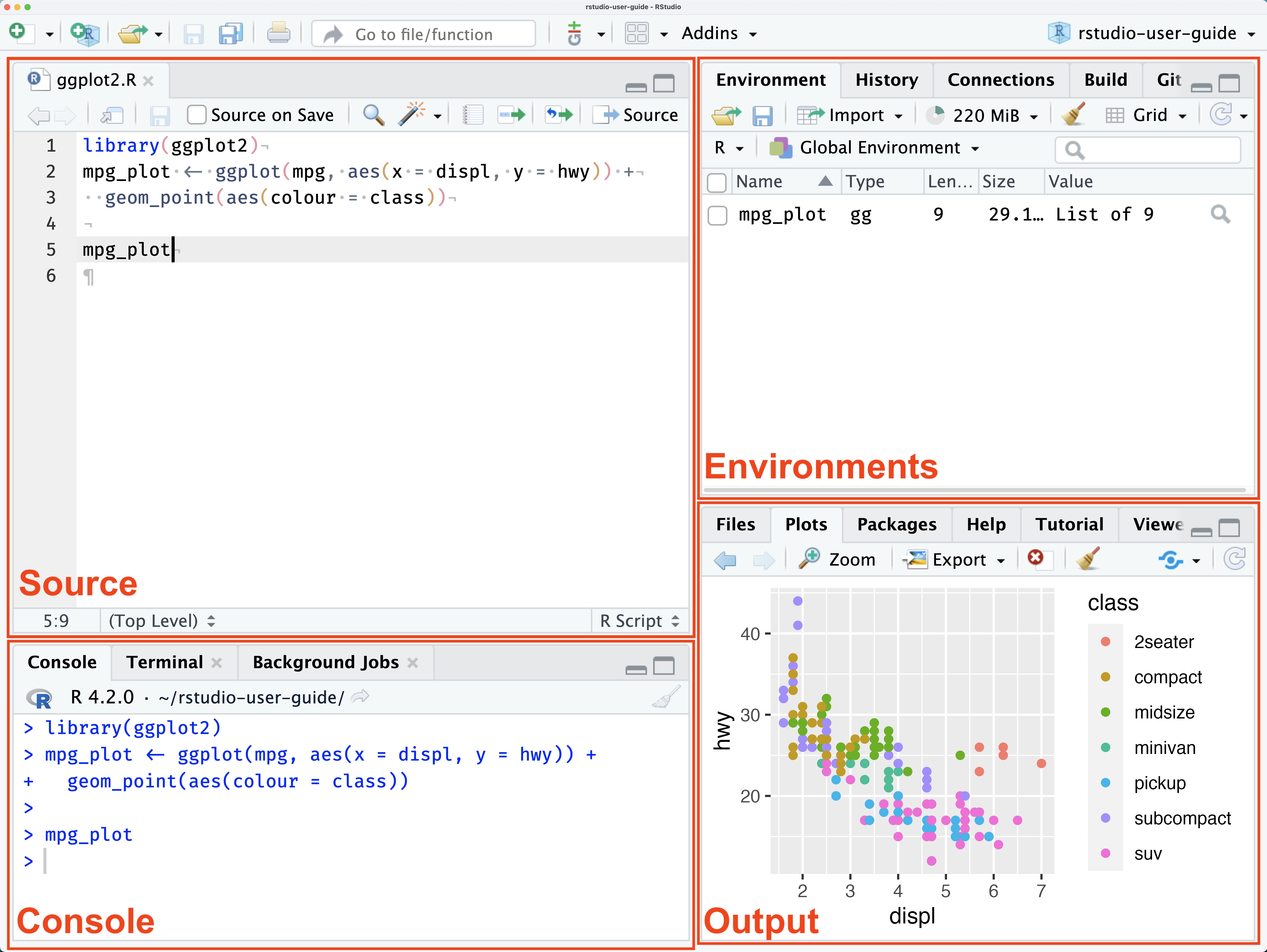
RStudio is an integrated development environment (IDE) for R, Python, and reproducible publishing. Its default layout contains four panes:

Pane	Main purpose
Source	Write and edit scripts and Quarto documents.
Console	Send expressions directly to R and view immediate results.
Environment/History	Inspect objects and review previous commands.
Files/Plots/Packages/Help/Viewer	Navigate files, inspect graphics, manage packages, read documentation, and preview output.

Use the console for short experiments. Any computation that matters should be placed in an R script or Quarto document so that it can be reproduced.

Figure 1.1: RStudio layout borrow from the Posit website.

1.2.2 R scripts and Quarto documents

An R script is a plain-text file with the extension .R. It contains R expressions that can be executed one line, one selection, or one file at a time.

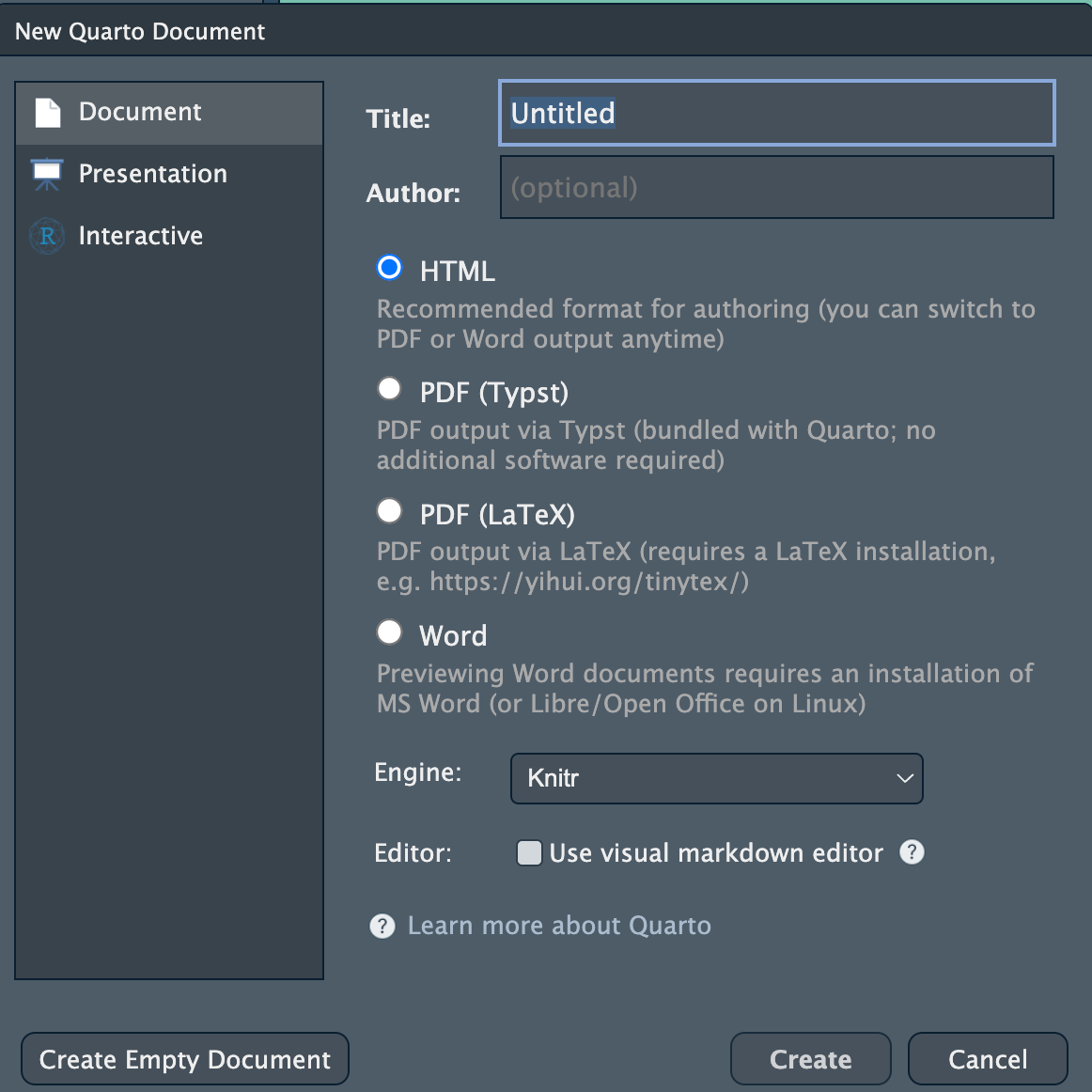
A Quarto document has the extension .qmd. It combines:

a YAML header describing the document;
prose written in Markdown;
executable code chunks;
tables, equations, figures, citations, and cross-references.

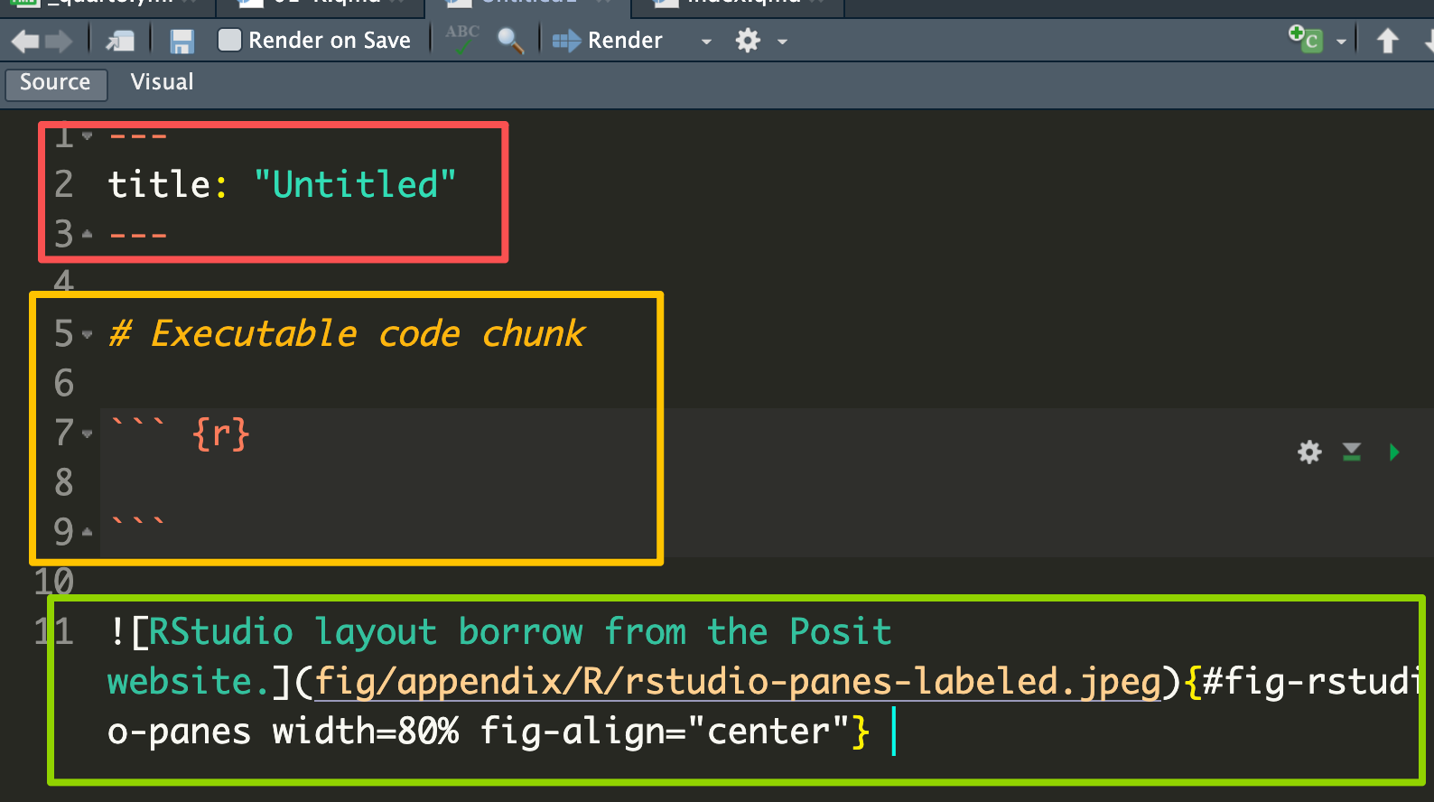
In Figure 1.3, the red box is the yaml, the yellow box is the executable code chunk and the green box is a figure.

For example, an executable R chunk is written as

```{r}
x <- rnorm(100)
mean(x)
```

[1] -0.01310165

Rendering the document executes the enabled chunks in order and places their results into the final output.

1.2.3 A project-oriented workflow

Create one RStudio Project for the course or for each substantial analysis. Use project-relative paths such as data/survey.csv rather than hard-coded paths tied to one computer.

A simple project might contain:

stat8670-project/
├── data/          # original and processed data
├── R/             # reusable functions
├── figures/       # saved figures
├── notes/         # Quarto lecture or analysis files
└── stat8670-project.Rproj

Avoid using setwd() inside a reproducible document. When a project is opened, its root provides a stable reference point for relative paths.

1.3 R as a computing environment

At the console, R follows a read, evaluate, print loop (REPL):

Read: parse the text entered by the user.
Evaluate: compute the value of the expression.
Print: display the result when appropriate.
Loop: wait for the next expression.

2 + 3 * 4

[1] 14

R respects operator precedence, so multiplication is performed before addition.

(2 + 3) * 4

[1] 20

Assignment usually returns its value invisibly:

x <- 2 + 3 * 4
x

[1] 14

A useful mental model

Most R code can be understood as functions operating on objects. Even operators such as + are functions.

`+`(2, 3)

[1] 5

1.4 Objects, data, and functions

Two fundamental kinds of objects that we will work with are:

Data objects
Functions

Data objects include numbers, vectors, matrices, arrays, lists, data frames, and fitted models.

A function is a set of instructions that receives input, performs a computation, and returns an output. Functions can be built into R, provided by a package, or written by the user.

mean(c(1, 2, 3, 4))

[1] 2.5

Here, c(1, 2, 3, 4) is a data object and mean() is a function.

1.5 Expressions, objects, and names

R computes with objects. A name is a symbol bound to an object.

sample_size <- 100
another_name <- sample_size

sample_size

[1] 100

another_name

[1] 100

The assignment operator <- creates or changes a binding.

Names are case-sensitive:

n <- 10
N <- 25

c(n = n, N = N)

 n  N 
10 25

A useful naming convention is to separate words using _:

sample_mean <- 10
number_students <- 30

Use ls() to list names in the current environment and rm() to remove a binding.

temporary_result <- 42
"temporary_result" %in% ls()

[1] TRUE

rm(temporary_result)

"temporary_result" %in% ls()

[1] FALSE

1.6 Data types

The fundamental data structure in R is the vector. An atomic vector contains elements of one common type.

Common atomic types include:

Type	Example	Typical use
logical	`TRUE`, `FALSE`	conditions and indicators
integer	`2L`	counts and indices
double	`2`, `3.14`	numerical computation
character	`"R"`	text and labels
complex	`1 + 2i`	complex arithmetic
raw	`charToRaw("R")`	bytes

logical_vector <- c(TRUE, FALSE, TRUE)
integer_vector <- c(1L, 2L, 3L)
double_vector <- c(1, 2, 3)
character_vector <- c("one", "two", "three")

typeof(logical_vector)

[1] "logical"

typeof(integer_vector)

[1] "integer"

typeof(double_vector)

[1] "double"

typeof(character_vector)

[1] "character"

1.6.1 Changing data types

Data types can be explicitly converted, but conversion may result in information loss.

x <- pi
x

[1] 3.141593

x_int <- as.integer(x)
x_int

[1] 3

Here, converting \(\pi\) to an integer removes its decimal component.

Common conversion functions include:

as.integer()
as.numeric()
as.character()
as.logical()
as.Date()
as.factor()
as.list()
as.matrix()
as.data.frame()
as.vector()
as.complex()

Type conversion can lose information

Always inspect the result after converting an object from one type to another.

1.7 Operators

A unary operator operates on one object:

-x
!x

A binary operator operates on two objects:

x + y
x - y
x * y
x / y

Comparison operators

Comparison operators return logical values:

x == y
x != y
x < y
x > y
x <= y
x >= y

Logical operators

Logical operators combine logical values:

x & y
x | y
!x

The operators & and | operate element by element.

x <- c(TRUE, FALSE, FALSE)
y <- c(TRUE, TRUE, FALSE)

x | y

[1]  TRUE  TRUE FALSE

x & y

[1]  TRUE FALSE FALSE

By contrast, && and || are intended for a single logical condition and are commonly used inside if statements.

1.8 Vectorization

Many R functions and operators act on entire vectors.

x <- c(1, 2, 3, 4)

x^2

[1]  1  4  9 16

sqrt(x)

[1] 1.000000 1.414214 1.732051 2.000000

sum(x)

[1] 10

mean(x)

[1] 2.5

Vectorized code often expresses statistical calculations more directly than element-by-element code.

1.9 Recycling

Arithmetic between vectors is usually element-wise.

x <- c(10, 20, 30)
y <- c(1, 2, 3)

x + y

[1] 11 22 33

If one vector is shorter, R may recycle its values.

c(10, 20, 30, 40) + c(1, 2)

[1] 11 22 31 42

When the shorter length does not divide the longer length exactly, R produces a warning.

c(10, 20, 30, 40) + c(1, 2, 3)

Warning in c(10, 20, 30, 40) + c(1, 2, 3): longer object length is not a
multiple of shorter object length

[1] 11 22 33 41

1.10 Coercion

An atomic vector must have one type. Combining different types may cause R to convert values to a common type.

mixed_numeric <- c(TRUE, 2L, 3.5)
mixed_character <- c(TRUE, 2L, 3.5, "four")

mixed_numeric

[1] 1.0 2.0 3.5

typeof(mixed_numeric)

[1] "double"

mixed_character

[1] "TRUE" "2"    "3.5"  "four"

typeof(mixed_character)

[1] "character"

A simplified coercion hierarchy is:

logical → integer → double → complex → character

Inspect unfamiliar objects using

typeof()
class()
length()
str()

1.11 Missing and special values

R uses NA to represent a missing value.

day <- c("Monday", "Tuesday", "Wednesday", "Thursday", "Friday")
weather <- c("Raining", "Sunny", NA, "Windy", "Snowing")

weather_data <- data.frame(day, weather)
weather_data

        day weather
1    Monday Raining
2   Tuesday   Sunny
3 Wednesday    <NA>
4  Thursday   Windy
5    Friday Snowing

Missing values usually propagate through calculations:

scores <- c(88, NA, 91, 84)

mean(scores)

[1] NA

mean(scores, na.rm = TRUE)

[1] 87.66667

is.na(scores)

[1] FALSE  TRUE FALSE FALSE

Do not use

x == NA

to detect missing values. Use

is.na(x)

instead.

Other special numerical values include

c(1 / 0, -1 / 0, 0 / 0)

[1]  Inf -Inf  NaN

which produce Inf, -Inf, and NaN.

1.12 Indexing and subsetting

Indexing allows us to access or modify parts of an object.

R indexing begins at 1

Unlike languages such as Python and C++, R uses 1-based indexing. The first element is indexed by 1, not 0.

For a vector:

x <- c(first = 10, second = 20, third = 30, fourth = 40)

x[1]

first 
   10

x[c(1, 3)]

first third 
   10    30

x[-2]

 first  third fourth 
    10     30     40

x[x >= 30]

 third fourth 
    30     40

x[c("second", "fourth")]

second fourth 
    20     40

Positive integers select positions, negative integers exclude positions, logical values filter positions, and character values select named elements.

A common surprise

Prefer seq_along(x) to 1:length(x) when iterating over the positions of an object.

empty <- numeric(0)

1:length(empty)

[1] 1 0

seq_along(empty)

integer(0)

1.13 Naming elements

Names can be attached to vector elements:

temp <- c(20, 30, 27, 31, 45)

names(temp) <- c("Mon", "Tues", "Wed", "Thurs", "Fri")

temp

  Mon  Tues   Wed Thurs   Fri 
   20    30    27    31    45

temp["Wed"]

Wed 
 27

A vector does not have rows, so this is inappropriate:

rownames(temp) <- "Day1"

A matrix can have row and column names:

temp_mat <- matrix(c(20, 30, 27, 31, 45),
                   nrow = 1,
                   ncol = 5)

colnames(temp_mat) <- c("Mon", "Tues", "Wed", "Thurs", "Fri")
rownames(temp_mat) <- "Day1"

temp_mat

     Mon Tues Wed Thurs Fri
Day1  20   30  27    31  45

1.14 Arrays and matrices

An array is a multidimensional data structure.

array_1d <- array(1:10, dim = 10)
array_1d

 [1]  1  2  3  4  5  6  7  8  9 10

array_2d <- array(1:12, dim = c(4, 3))
array_2d

     [,1] [,2] [,3]
[1,]    1    5    9
[2,]    2    6   10
[3,]    3    7   11
[4,]    4    8   12

array_3d <- array(1:24, dim = c(4, 3, 2))
array_3d

, , 1

     [,1] [,2] [,3]
[1,]    1    5    9
[2,]    2    6   10
[3,]    3    7   11
[4,]    4    8   12

, , 2

     [,1] [,2] [,3]
[1,]   13   17   21
[2,]   14   18   22
[3,]   15   19   23
[4,]   16   20   24

A matrix is a two-dimensional array:

my_matrix <- matrix(1:12, nrow = 4, ncol = 3)
my_matrix

     [,1] [,2] [,3]
[1,]    1    5    9
[2,]    2    6   10
[3,]    3    7   11
[4,]    4    8   12

is.matrix(array_2d)

[1] TRUE

is.matrix(my_matrix)

[1] TRUE

is.array(array_2d)

[1] TRUE

is.array(my_matrix)

[1] TRUE

A matrix is an atomic vector with a dim attribute, so all entries must share one common type.

A <- matrix(1:6, nrow = 2, ncol = 3)

attributes(A)

$dim
[1] 2 3

A[2, 3]

[1] 6

Matrix multiplication uses %*%:

B <- matrix(c(1, 0, 0, 1, 1, 1), nrow = 3)

A %*% B

     [,1] [,2]
[1,]    1    9
[2,]    2   12

while * performs element-wise multiplication.

1.15 Lists and key-value pairs

A list can contain objects of different types and lengths.

fit_summary <- list(
  method = "least squares",
  coefficients = c(intercept = 1.2, slope = 0.8),
  converged = TRUE
)

str(fit_summary)

List of 3
 $ method      : chr "least squares"
 $ coefficients: Named num [1:2] 1.2 0.8
  ..- attr(*, "names")= chr [1:2] "intercept" "slope"
 $ converged   : logi TRUE

Named list elements naturally form key-value pairs.

key1 <- "Tues"
value1 <- 32

key2 <- "Wed"
value2 <- 28

list_temp <- list()

list_temp[[key1]] <- value1
list_temp[[key2]] <- value2

list_temp

$Tues
[1] 32

$Wed
[1] 28

Values can then be obtained from their keys:

list_temp[["Tues"]]

[1] 32

list_temp$Tues

[1] 32

For lists, note the important distinction:

fit_summary["coefficients"]

$coefficients
intercept     slope 
      1.2       0.8

fit_summary[["coefficients"]]

intercept     slope 
      1.2       0.8

[ returns a sublist, whereas [[ extracts the element itself.

1.16 Factors

A factor represents categorical data using integer codes and a set of levels.

group <- factor(c("control", "treatment", "control"))

group

[1] control   treatment control  
Levels: control treatment

unclass(group)

[1] 1 2 1
attr(,"levels")
[1] "control"   "treatment"

levels(group)

[1] "control"   "treatment"

The order of factor levels matters in statistical models, so define it deliberately when necessary.

1.17 Data frames

A data frame is a two-dimensional rectangular data structure.

Conceptually, a data frame is a named list of equal-length vectors:

each row represents an observational unit;
each column represents a variable;
columns may have different data types.

students <- data.frame(
  id = 1:6,
  name = c("Alice", "Bob", "Chen", "Divya", "Elena", "Farah"),
  program = c("MS", "PhD", "MS", "PhD", "MS", "PhD"),
  score = c(90, 85, NA, 94, 88, 91),
  completed = c(TRUE, TRUE, FALSE, TRUE, TRUE, TRUE)
)

students

  id  name program score completed
1  1 Alice      MS    90      TRUE
2  2   Bob     PhD    85      TRUE
3  3  Chen      MS    NA     FALSE
4  4 Divya     PhD    94      TRUE
5  5 Elena      MS    88      TRUE
6  6 Farah     PhD    91      TRUE

Another familiar built-in data frame is:

iris <- datasets::iris
head(iris)

  Sepal.Length Sepal.Width Petal.Length Petal.Width Species
1          5.1         3.5          1.4         0.2  setosa
2          4.9         3.0          1.4         0.2  setosa
3          4.7         3.2          1.3         0.2  setosa
4          4.6         3.1          1.5         0.2  setosa
5          5.0         3.6          1.4         0.2  setosa
6          5.4         3.9          1.7         0.4  setosa

1.17.1 Inspecting a data frame

Always inspect newly imported data before analyzing them.

class(students)

[1] "data.frame"

dim(students)

[1] 6 5

nrow(students)

[1] 6

ncol(students)

[1] 5

names(students)

[1] "id"        "name"      "program"   "score"     "completed"

str(students)

'data.frame':   6 obs. of  5 variables:
 $ id       : int  1 2 3 4 5 6
 $ name     : chr  "Alice" "Bob" "Chen" "Divya" ...
 $ program  : chr  "MS" "PhD" "MS" "PhD" ...
 $ score    : num  90 85 NA 94 88 91
 $ completed: logi  TRUE TRUE FALSE TRUE TRUE TRUE

summary(students)

       id              name        program      score      completed      
 Min.   :1.00   Length   :6   Length   :6   Min.   :85.0   Mode :logical  
 1st Qu.:2.25   N.unique :6   N.unique :2   1st Qu.:88.0   FALSE:1        
 Median :3.50   N.blank  :0   N.blank  :0   Median :90.0   TRUE :5        
 Mean   :3.50   Min.nchar:3   Min.nchar:2   Mean   :89.6                  
 3rd Qu.:4.75   Max.nchar:5   Max.nchar:3   3rd Qu.:91.0                  
 Max.   :6.00                               Max.   :94.0                  
                                            NAs    :1

head(students, 3)

  id  name program score completed
1  1 Alice      MS    90      TRUE
2  2   Bob     PhD    85      TRUE
3  3  Chen      MS    NA     FALSE

str() is especially useful because it gives a compact summary of the object’s structure and types.

1.17.2 Subsetting a data frame

Use

data[rows, columns]

for two-dimensional indexing:

students[1, ]

  id  name program score completed
1  1 Alice      MS    90      TRUE

students[, c("name", "score")]

   name score
1 Alice    90
2   Bob    85
3  Chen    NA
4 Divya    94
5 Elena    88
6 Farah    91

students[students$program == "PhD", ]

  id  name program score completed
2  2   Bob     PhD    85      TRUE
4  4 Divya     PhD    94      TRUE
6  6 Farah     PhD    91      TRUE

students[1:3, c("name", "score")]

   name score
1 Alice    90
2   Bob    85
3  Chen    NA

students[2, "score"]

[1] 85

Three commonly used ways to extract a column are:

students["score"]

students[["score"]]

[1] 90 85 NA 94 88 91

students$score

[1] 90 85 NA 94 88 91

The first returns a one-column data frame. The latter two return the underlying vector.

1.17.3 Adding and modifying variables

students$passed <- students$score >= 70

students$centered_score <-
  students$score - mean(students$score, na.rm = TRUE)

students

  id  name program score completed passed centered_score
1  1 Alice      MS    90      TRUE   TRUE            0.4
2  2   Bob     PhD    85      TRUE   TRUE           -4.6
3  3  Chen      MS    NA     FALSE     NA             NA
4  4 Divya     PhD    94      TRUE   TRUE            4.4
5  5 Elena      MS    88      TRUE   TRUE           -1.6
6  6 Farah     PhD    91      TRUE   TRUE            1.4

Missingness propagates naturally. If a score is unknown, whether the student passed is also unknown.

1.17.4 Importing rectangular data

survey <- read.csv(
  "data/survey.csv",
  na.strings = c("", "NA", ".")
)

measurements <- read.table(
  "data/measurements.txt",
  header = TRUE,
  sep = "\t"
)

After importing, check:

dim(survey)
names(survey)
str(survey)
head(survey)
colSums(is.na(survey))

Data import is part of the analysis

Import settings such as delimiters, missing-value codes, decimal marks, encodings, and inferred variable types can change the data that R sees and therefore affect the final analysis.

Do not automatically treat a data frame as a matrix

apply() first converts a data frame to a matrix. A mixed-type data frame can therefore be converted entirely to character values. Use lapply(), vapply(), or dplyr::across() for column-wise operations when types differ.

1.18 Functions

A function packages a computation so that it can be reused.

standardize <- function(x, remove_na = FALSE) {
  center <- mean(x, na.rm = remove_na)
  spread <- sd(x, na.rm = remove_na)

  (x - center) / spread
}

standardize(c(2, 4, 6, 8))

[1] -1.1618950 -0.3872983  0.3872983  1.1618950

A function has three main components:

formals: the arguments;
body: the expressions evaluated;
environment: where the function was created.

formals(standardize)

$x


$remove_na
[1] FALSE

body(standardize)

{
    center <- mean(x, na.rm = remove_na)
    spread <- sd(x, na.rm = remove_na)
    (x - center)/spread
}

environment(standardize)

<environment: R_GlobalEnv>

When a function is called, R creates a temporary environment, matches the arguments, evaluates the body, and returns the value of the final expression unless return() is called earlier.

1.18.1 Argument matching

Arguments can be matched by name or position.

round(x = 3.14159, digits = 3)

[1] 3.142

round(3.14159, 3)

[1] 3.142

Named arguments are often clearer in code intended to be read by others.

1.18.2 Lazy evaluation

R evaluates function arguments only when they are needed.

choose_one <- function(x, y) {
  x
}

choose_one(
  10,
  stop("This argument is never evaluated")
)

[1] 10

This behavior is called lazy evaluation.

1.19 Environments and lexical scoping

An environment stores name-object bindings and has a parent environment.

R uses lexical scoping: functions look for nonlocal names in the environment where they were defined.

make_power <- function(power) {
  function(x) {
    x^power
  }
}

square <- make_power(2)
cube <- make_power(3)

square(5)

[1] 25

cube(5)

[1] 125

A function together with its defining environment is called a closure.

Local assignment affects the current function environment:

x <- 100

change_locally <- function() {
  x <- 5
  x
}

change_locally()

[1] 5

[1] 100

1.20 Memory and copy-on-modify

R behaves as if objects are copied when modified.

x <- c(10, 20, 30)
y <- x

y[1] <- 999

x

[1] 10 20 30

[1] 999  20  30

Changing y does not change x.

Repeatedly expanding an object can require many allocations:

result <- numeric(0)

for (i in seq_len(100000)) {
  result <- c(result, i^2)
}

Instead, preallocate the required memory:

n <- 100000

result <- numeric(n)

for (i in seq_len(n)) {
  result[i] <- i^2
}

head(result)

[1]  1  4  9 16 25 36

1.21 Iteration: vectorization, loops, and the apply family

An iterative computation can usually be expressed in several ways.

x <- c(2, 4, 6, 8)

# Vectorized
x^2

[1]  4 16 36 64

# Preallocated loop
squares <- numeric(length(x))

for (i in seq_along(x)) {
  squares[i] <- x[i]^2
}

squares

[1]  4 16 36 64

# Apply a function
vapply(
  x,
  function(value) value^2,
  numeric(1)
)

[1]  4 16 36 64

Use vectorization when an existing vectorized function directly expresses the computation. Use a loop when the calculation has evolving state or complex indexing. Use an apply-family function when the same operation is independently applied to several pieces of an object.

The apply family is not magic vectorization

apply() and lapply() still perform iteration internally. They are not automatically faster than a well-written preallocated for loop. Their main advantage is often clarity and conciseness.

1.21.1 `apply()`

apply(X, MARGIN, FUN, ...) applies a function over dimensions of a matrix or array.

MARGIN = 1: rows
MARGIN = 2: columns

X <- matrix(1:12, nrow = 3, byrow = TRUE)

colnames(X) <- c("x1", "x2", "x3", "x4")

X

     x1 x2 x3 x4
[1,]  1  2  3  4
[2,]  5  6  7  8
[3,]  9 10 11 12

apply(X, MARGIN = 1, FUN = mean)

[1]  2.5  6.5 10.5

apply(X, MARGIN = 2, FUN = sd)

x1 x2 x3 x4 
 4  4  4  4

Additional arguments are passed through ...:

X_missing <- X
X_missing[2, 3] <- NA

apply(X_missing, 2, mean, na.rm = TRUE)

x1 x2 x3 x4 
 5  6  7  8

For common operations, specialized functions are preferable:

rowMeans(X)

[1]  2.5  6.5 10.5

colMeans(X)

x1 x2 x3 x4 
 5  6  7  8

rowSums(X)

[1] 10 26 42

colSums(X)

x1 x2 x3 x4 
15 18 21 24

1.21.2 Why `apply()` can be dangerous for data frames

mixed_df <- data.frame(
  id = c("A", "B", "C"),
  x = c(10, 20, 30),
  y = c(2, 4, 6)
)

as.matrix(mixed_df)

     id  x    y  
[1,] "A" "10" "2"
[2,] "B" "20" "4"
[3,] "C" "30" "6"

typeof(as.matrix(mixed_df))

[1] "character"

Because one column is character, the entire matrix becomes character.

A safer approach is:

numeric_columns <- vapply(
  mixed_df,
  is.numeric,
  logical(1)
)

vapply(
  mixed_df[numeric_columns],
  mean,
  numeric(1)
)

 x  y 
20  4

1.21.3 `lapply()`

lapply() applies a function to each element and always returns a list.

lapply(students, class)

$id
[1] "integer"

$name
[1] "character"

$program
[1] "character"

$score
[1] "numeric"

$completed
[1] "logical"

$passed
[1] "logical"

$centered_score
[1] "numeric"

lapply(
  students[c("score", "centered_score")],
  mean,
  na.rm = TRUE
)

$score
[1] 89.6

$centered_score
[1] 5.861978e-15

1.21.4 `sapply()` and `vapply()`

sapply() attempts to simplify the output.

sapply(students, class)

            id           name        program          score      completed 
     "integer"    "character"    "character"      "numeric"      "logical" 
        passed centered_score 
     "logical"      "numeric"

vapply() requires the expected output type:

vapply(students, typeof, character(1))

            id           name        program          score      completed 
     "integer"    "character"    "character"       "double"      "logical" 
        passed centered_score 
     "logical"       "double"

This makes vapply() safer for reusable code.

1.21.5 `tapply()`

tapply() splits a vector into groups and applies a function within each group.

with(
  students,
  tapply(score, program, mean, na.rm = TRUE)
)

 MS PhD 
 89  90

1.21.6 `Map()` and `mapply()`

These functions apply a function to corresponding elements of multiple inputs.

Map(
  function(center, spread) rnorm(3, center, spread),
  center = c(0, 10),
  spread = c(1, 2)
)

[[1]]
[1]  0.2896038  1.4751528 -0.2142565

[[2]]
[1] 13.124713 11.324494  6.852467

1.21.7 Choosing an iteration tool

Goal	Recommended starting point
Element-wise arithmetic	Vectorized function or operator
Standard matrix row/column summaries	`rowSums()`, `colSums()`, `rowMeans()`, `colMeans()`
General matrix row/column operation	`apply()`
Operation on list or data-frame columns	`lapply()`
Known scalar output type	`vapply()`
Grouped operation on one vector	`tapply()`
Data-frame columns in tidyverse	`dplyr::across()`
Complex state-dependent computation	Preallocated `for` loop

1.22 Packages and help

Packages extend R with functions, data, documentation, and statistical methods. The historical package count can be found https://www.datasciencemeta.com/rpackages.

# CRAN
install.packages("packageName")

# Bioconductor
BiocManager::install("packageName")

# GitHub
remotes::install_github("username/repository")

Load an installed package:

library(packageName)

or call one function explicitly:

packageName::function_name()

Useful help tools include:

?mean
help("mean")
example(mean)
args(mean)
methods(mean)

1.23 The tidyverse

The tidyverse is a coordinated collection of R packages for data manipulation, visualization, importing, tidying, and programming.

install.packages("tidyverse")

library(tidyverse)

Important packages include:

library(dplyr)    # data manipulation
library(ggplot2)  # data visualization
library(readr)    # data import
library(tibble)   # tidy data frames
library(tidyr)    # data tidying
library(purrr)    # functional programming

Base R and tidyverse tools are complementary rather than competing systems.

1.23.1 Data frames and tibbles

A tibble is a modern data frame.

students_tbl <- as_tibble(students)

students_tbl

# A tibble: 6 × 7
     id name  program score completed passed centered_score
  <int> <chr> <chr>   <dbl> <lgl>     <lgl>           <dbl>
1     1 Alice MS         90 TRUE      TRUE            0.400
2     2 Bob   PhD        85 TRUE      TRUE           -4.60 
3     3 Chen  MS         NA FALSE     NA             NA    
4     4 Divya PhD        94 TRUE      TRUE            4.40 
5     5 Elena MS         88 TRUE      TRUE           -1.60 
6     6 Farah PhD        91 TRUE      TRUE            1.40

class(students_tbl)

[1] "tbl_df"     "tbl"        "data.frame"

Some important differences are:

Operation	Base data frame	Tibble
Printing	May print many rows	Compact preview
`x[, "score"]`	May simplify	Remains a tibble
Partial matching	May occur in some contexts	More strict
Row names	Supported	Discouraged

Both are still data frames:

is.data.frame(students_tbl)

[1] TRUE

1.23.2 Pipe operators

The native R pipe is

|>

and the commonly used magrittr/tidyverse pipe is

%>%

The pipe passes the result of one operation to the next function.

set.seed(777)

x <- rnorm(5)

# Without pipe
print(round(mean(x), 2))

[1] 0.37

# Native pipe
x |>
  mean() |>
  round(2) |>
  print()

[1] 0.37

The pipe makes the sequence of operations explicit.

A useful formatting rule is that |> should have spaces around it and normally appear at the end of a line.

1.23.3 Core `dplyr` verbs

Verb	Purpose
`select()`	Choose or reorder columns
`filter()`	Retain rows satisfying conditions
`arrange()`	Sort observations
`mutate()`	Create or modify variables
`summarise()`	Compute summaries
`group_by()`	Define groups

Example:

students_tbl |>
  filter(completed, !is.na(score)) |>
  select(name, program, score) |>
  arrange(desc(score))

# A tibble: 5 × 3
  name  program score
  <chr> <chr>   <dbl>
1 Divya PhD        94
2 Farah PhD        91
3 Alice MS         90
4 Elena MS         88
5 Bob   PhD        85

Create variables and summarize by group:

students_tbl |>
  mutate(
    passed = score >= 70,
    score_z =
      (score - mean(score, na.rm = TRUE)) /
      sd(score, na.rm = TRUE)
  ) |>
  group_by(program) |>
  summarise(
    n = n(),
    n_observed = sum(!is.na(score)),
    mean_score = mean(score, na.rm = TRUE),
    sd_score = sd(score, na.rm = TRUE),
    .groups = "drop"
  )

# A tibble: 2 × 5
  program     n n_observed mean_score sd_score
  <chr>   <int>      <int>      <dbl>    <dbl>
1 MS          3          2         89     1.41
2 PhD         3          3         90     4.58

1.23.4 Applying functions across several columns

Inside mutate() or summarise(), across() applies functions to selected columns.

students_tbl |>
  summarise(
    across(
      where(is.numeric),
      list(
        mean = ~ mean(.x, na.rm = TRUE),
        sd = ~ sd(.x, na.rm = TRUE)
      ),
      .names = "{.col}_{.fn}"
    )
  )

# A tibble: 1 × 6
  id_mean id_sd score_mean score_sd centered_score_mean centered_score_sd
    <dbl> <dbl>      <dbl>    <dbl>               <dbl>             <dbl>
1     3.5  1.87       89.6     3.36            5.86e-15              3.36

This provides a tidyverse alternative to column-wise lapply() or vapply().

1.24 Base R and tidyverse are complementary

For example, the same grouped mean can be obtained using either style.

# Base R
aggregate(
  score ~ program,
  data = students,
  FUN = mean,
  na.rm = TRUE
)

  program score
1      MS    89
2     PhD    90

# tidyverse
students_tbl |>
  group_by(program) |>
  summarise(
    mean_score = mean(score, na.rm = TRUE),
    .groups = "drop"
  )

# A tibble: 2 × 2
  program mean_score
  <chr>        <dbl>
1 MS              89
2 PhD             90

The important questions are the same regardless of syntax:

What object enters the function?
What object does the function return?
How are missing values handled?
Are types and groups preserved?

1.25 Numerical computation and finite precision

Most real numbers cannot be represented exactly using binary floating-point arithmetic.

0.1 + 0.2

[1] 0.3

(0.1 + 0.2) == 0.3

[1] FALSE

all.equal(0.1 + 0.2, 0.3)

[1] TRUE

For computed floating-point quantities, tolerance-based comparisons such as all.equal() are usually more appropriate than exact equality.

Numerical algorithms must also consider overflow, underflow, cancellation, conditioning, and convergence.

log(dbinom(500, size = 1000, prob = 0.01))

[1] -Inf

dbinom(
  500,
  size = 1000,
  prob = 0.01,
  log = TRUE
)

[1] -1618.143

The second computation is numerically safer.

1.26 Randomness and reproducibility

Pseudo-random numbers are generated deterministically from an internal state.

set.seed(8670)
rnorm(5)

[1] -0.4916281  1.1467524  1.5963118 -0.6655463  0.5516107

set.seed(8670)
rnorm(5)

[1] -0.4916281  1.1467524  1.5963118 -0.6655463  0.5516107

The two results are identical.

Set the seed at a meaningful boundary, usually once near the beginning of a simulation, rather than repeatedly inside the simulation loop.

Record the information necessary to reproduce the analysis:

sessionInfo()

R version 4.6.0 (2026-04-24)
Platform: aarch64-apple-darwin23
Running under: macOS Tahoe 26.6.2

Matrix products: default
BLAS:   /Library/Frameworks/R.framework/Versions/4.6/Resources/lib/libRblas.0.dylib 
LAPACK: /Library/Frameworks/R.framework/Versions/4.6/Resources/lib/libRlapack.dylib;  LAPACK version 3.12.1

locale:
[1] en_US.UTF-8/en_US.UTF-8/en_US.UTF-8/C/en_US.UTF-8/en_US.UTF-8

time zone: America/New_York
tzcode source: internal

attached base packages:
[1] stats     graphics  grDevices utils     datasets  methods   base     

other attached packages:
 [1] lubridate_1.9.5 forcats_1.0.1   stringr_1.6.0   dplyr_1.2.1    
 [5] purrr_1.2.2     readr_2.2.0     tidyr_1.3.2     tibble_3.3.1   
 [9] ggplot2_4.0.3   tidyverse_2.0.0

loaded via a namespace (and not attached):
 [1] gtable_0.3.6       jsonlite_2.0.0     compiler_4.6.0     tidyselect_1.2.1  
 [5] scales_1.4.0       yaml_2.3.12        fastmap_1.2.0      R6_2.6.1          
 [9] generics_0.1.4     knitr_1.51         htmlwidgets_1.6.4  pillar_1.11.1     
[13] RColorBrewer_1.1-3 tzdb_0.5.0         rlang_1.3.0        utf8_1.2.6        
[17] stringi_1.8.9      xfun_0.60          S7_0.2.2           otel_0.2.0        
[21] timechange_0.4.0   cli_3.6.6          withr_3.0.3        magrittr_2.0.5    
[25] digest_0.6.39      grid_4.6.0         rstudioapi_0.19.0  hms_1.1.4         
[29] lifecycle_1.0.5    vctrs_0.7.3        evaluate_1.0.5     glue_1.8.1        
[33] farver_2.1.2       codetools_0.2-20   rmarkdown_2.31     tools_4.6.0       
[37] pkgconfig_2.0.3    htmltools_0.5.9

1.27 Debugging and error messages

When an error occurs:

Read the entire error message.
Reduce the problem to the smallest example that still fails.
Inspect objects with str(), typeof(), class(), and dim().
Use traceback() after an error when necessary.
Verify assumptions with functions such as stopifnot().

safe_mean <- function(x) {
  stopifnot(
    is.numeric(x),
    length(x) > 0
  )

  mean(x)
}

safe_mean(c(2, 4, 6))

[1] 4

1.28 A computational workflow for this course

A reliable statistical computation separates:

Inputs: data, constants, configuration, and random seeds.
Transformation: cleaning and constructing analysis variables.
Computation: algorithms, models, optimization, or simulation.
Validation: diagnostics, tests, and sensitivity analysis.
Communication: figures, tables, interpretation, and limitations.

For example:

set.seed(8670)

n <- 200

x <- rnorm(n)
y <- 1 + 2 * x + rnorm(n, sd = 0.75)

simulated_data <- data.frame(
  x = x,
  y = y
)

fit <- lm(y ~ x, data = simulated_data)

coef(fit)

(Intercept)           x 
   1.020794    1.991843

This script records where the data came from, fixes the random seed, creates an explicit data object, and passes that object to the statistical model.

1.29 In-class exercises

Predict the value and type of each expression before running the code.

c(TRUE, 2L, 3.5)

c(1, 2, 3, 4) + c(10, 20)

c(1, 2, NA) > 1

TRUE | NA

Using

x <- c(4, NA, 10, 15, 3, NA, 21)

write expressions that return:

all nonmissing values;
values greater than or equal to 10;
the positions of values greater than or equal to 10;
the mean of the observed values.

Without running the code, determine the result of f(5) and identify where each occurrence of a is found.

a <- 10

f <- function(x) {
  a <- 2

  g <- function(y) {
    a * y
  }

  g(x)
}

f(5)

Write a function that takes a positive integer n and returns a vector whose \(i\)th element is

\[ \frac{(-1)^{i+1}}{i}. \]

Preallocate the result and use seq_len(n).

Using students, complete each task once with base R and once with dplyr:

retain students with observed scores;
select name, program, and score;
create a variable equal to score - 90;
sort from highest to lowest score;
compute the number of observed scores and mean score within each program.

Before running the code, predict whether each result is a vector, data frame, tibble, or grouped tibble.

For each task, choose among a vectorized function, apply(), lapply(), vapply(), tapply(), dplyr::across(), or a loop. Justify your choice and then write the code.

Compute the mean of every numeric column in students.
Compute the row sums of a \(10,000\times50\) numerical matrix.
Record the class of every column in a data frame.
Compute the mean score within each program.
Fit the same model to each of 20 independently generated data sets and retain the fitted-model objects.

Predict the type and contents of result. Explain why apply() is inappropriate and rewrite the computation using vapply() or dplyr::across().

dat <- data.frame(
  subject = c("A", "B", "C"),
  pre = c(10, 12, 9),
  post = c(14, 13, 15)
)

result <- apply(dat, 2, mean)

1.30 Takeaways

R is both a programming language and an environment for statistical computing.
Objects and functions are the basic building blocks of R programs.
Atomic vectors are the foundation of R computation.
R uses 1-based indexing.
Vectorization, recycling, coercion, and missing-value propagation are central features of R.
Matrices and arrays require homogeneous element types, whereas lists can contain heterogeneous objects.
A data frame is a named list of equal-length columns.
Tibbles are modern data frames with stricter and more predictable behavior.
Functions have arguments, a body, and an environment.
R uses lexical scoping and lazy evaluation.
The apply family provides convenient abstractions for repeated computation but is not automatically faster than loops.
apply() is designed primarily for matrices and arrays and can cause unwanted coercion when applied to mixed-type data frames.
Base R and tidyverse tools are complementary.
The pipe (%>% or |>) can make a sequence of data transformations easier to read.
R’s copy-on-modify behavior gives objects intuitive semantics, although memory allocation still matters.
Statistical computing requires attention to floating-point arithmetic, missing values, reproducibility, and numerical stability.
Understanding R’s computational model makes code easier to predict, debug, optimize, and trust.

1.31 Optional challenge

Explain why these two functions may have very different memory and timing behavior even though they return the same values.

grow <- function(n) {
  out <- numeric(0)

  for (i in seq_len(n)) {
    out <- c(out, i^2)
  }

  out
}

preallocate <- function(n) {
  out <- numeric(n)

  for (i in seq_len(n)) {
    out[i] <- i^2
  }

  out
}

Design a timing experiment for increasing values of n.

Some of the materials are adapted from CMU Stat36-350.

A comprehensive reference for the tidyverse tools is R for Data Science.

A comprehensive reference for ggplot2 is ggplot2: Elegant Graphics for Data Analysis.

Additional introductory material is adapted from Why R?.