3  Optimization

Optimization plays an important role in statistical computing. Many statistical estimators can be written as

\[ \hat{\theta} = \arg\min_{\theta} Q(\theta) \qquad\text{or}\qquad \hat{\theta} = \arg\max_{\theta} \ell(\theta), \]

where \(Q(\theta)\) is an objective function and \(\ell(\theta)\) may be a likelihood.

For simple problems, a closed-form solution may exist. For many statistical models, however, the solution must be obtained numerically.

Examples include maximum likelihood estimation, nonlinear regression, mixture models, machine learning, smoothing, and regularization.

The central idea is

\[ \boxed{ \text{Statistical Problem} \Longleftrightarrow \text{Optimization Problem} \Longleftrightarrow \text{Numerical Algorithm} \Longleftrightarrow \text{R Implementation} }. \]

3.1 Why Numerical Optimization?

Consider

\[ X_1,\ldots,X_n \stackrel{iid}{\sim} N(\mu,1). \]

From mathematical statistics,

\[ \hat{\mu}_{MLE} = \bar X. \]

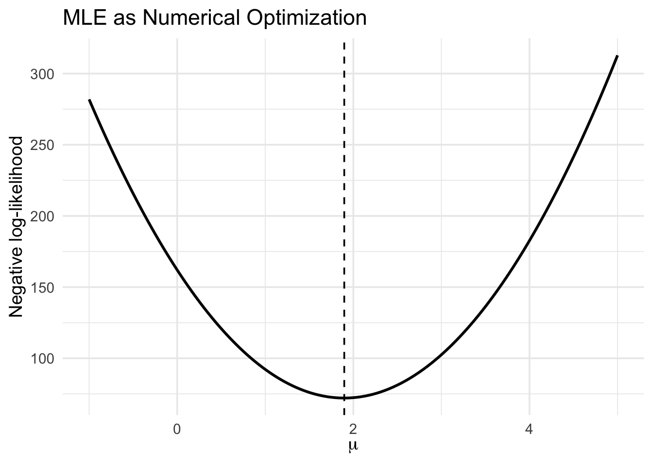
We already know the closed-form solution. However, we can also obtain the estimator computationally by minimizing the negative log-likelihood.

Code
set.seed(8670)

x <- rnorm(
  n = 50,
  mean = 2,
  sd = 1
)

nll <- function(mu) {
  -sum(
    dnorm(
      x,
      mean = mu,
      sd = 1,
      log = TRUE
    )
  )
}

fit <- optimize(
  nll,
  interval = c(-1, 5)
)

c(
  numerical = fit$minimum,
  theoretical = mean(x)
)
  numerical theoretical 
    1.89689     1.89689 

Visualizing the Objective Function

Rather than treating an optimizer as a black box, we can evaluate the objective function over a grid.

Code
mu_grid <- seq(
  -1,
  5,
  length.out = 400
)

nll_data <- data.frame(
  mu = mu_grid,
  nll = vapply(
    mu_grid,
    nll,
    numeric(1)
  )
)

ggplot(
  nll_data,
  aes(
    x = mu,
    y = nll
  )
) +
  geom_line(linewidth = 1) +
  geom_vline(
    xintercept = mean(x),
    linetype = "dashed"
  ) +
  labs(
    x = expression(mu),
    y = "Negative log-likelihood",
    title = "MLE as Numerical Optimization"
  )

Why is numerical optimization useful here if we already know that

\[ \hat{\mu}_{MLE}=\bar X? \]

The closed-form solution gives us a way to validate the numerical algorithm.

When a closed-form solution is unavailable, numerical optimization becomes essential.

3.2 When There Is No Closed-Form Solution

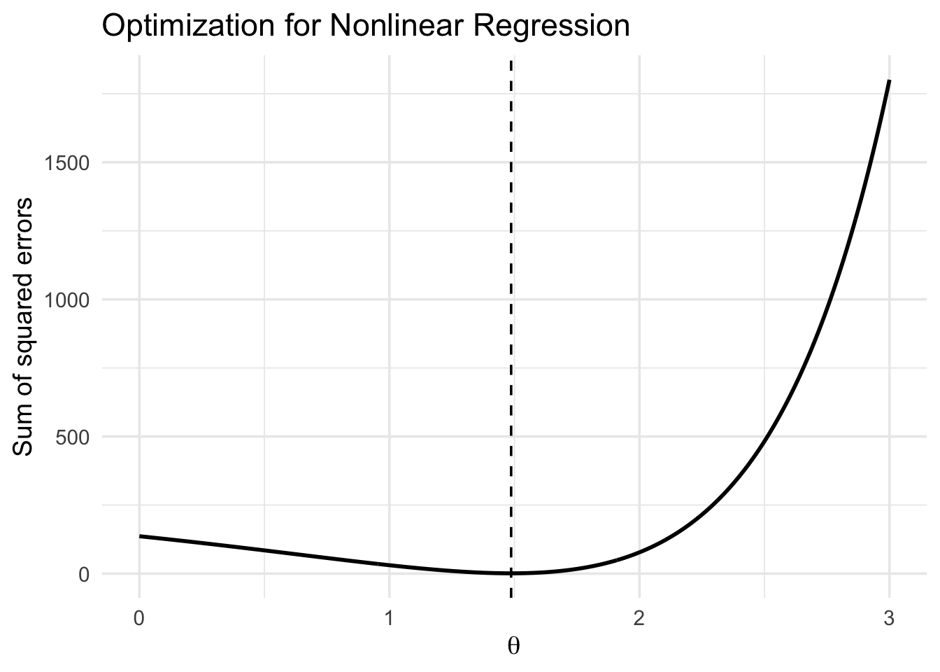
Consider the nonlinear regression model

\[ Y_i = \exp(\theta X_i) + \varepsilon_i. \]

Suppose we estimate \(\theta\) by minimizing

\[ Q(\theta) = \sum_{i=1}^n \left[ Y_i-\exp(\theta X_i) \right]^2. \]

Unlike ordinary linear regression, there is no convenient closed-form least-squares estimator.

Code
set.seed(8670)

x <- seq(
  0,
  1,
  length.out = 50
)

y <- exp(1.5 * x) +
  rnorm(
    50,
    sd = 0.15
  )

sse <- function(theta) {
  sum(
    (y - exp(theta * x))^2
  )
}

fit_nonlinear <- optimize(
  sse,
  interval = c(0, 3)
)

fit_nonlinear$minimum
[1] 1.486825
Code
theta_grid <- seq(
  0,
  3,
  length.out = 400
)

sse_data <- data.frame(
  theta = theta_grid,
  SSE = vapply(
    theta_grid,
    sse,
    numeric(1)
  )
)

ggplot(
  sse_data,
  aes(
    x = theta,
    y = SSE
  )
) +
  geom_line(linewidth = 1) +
  geom_vline(
    xintercept = fit_nonlinear$minimum,
    linetype = "dashed"
  ) +
  labs(
    x = expression(theta),
    y = "Sum of squared errors",
    title = "Optimization for Nonlinear Regression"
  )

The important distinction is

\[ \boxed{ \text{Theory tells us what to optimize;} \qquad \text{computation tells us how to find it.} } \]

3.3 Two Families of Optimization Methods

Computational optimization methods can be broadly divided into two families:

\[ \boxed{ \text{Deterministic Methods} \qquad\text{and}\qquad \text{Metaheuristic Methods}. } \]

3.3.1 Deterministic Methods

A deterministic algorithm follows a predictable sequence of updates once the starting value is fixed.

Examples include:

  • Newton’s method;
  • gradient descent;
  • quasi-Newton methods such as BFGS;
  • deterministic root-finding methods.

Advantages:

  • usually efficient for smooth and well-behaved problems;
  • mathematically well understood;
  • convergence can often be studied theoretically;
  • reproducible for a fixed starting value.

Limitations:

  • may converge to a local rather than global optimum;
  • can be sensitive to the starting value;
  • some methods require derivatives;
  • poor scaling can substantially slow convergence.

3.3.2 Metaheuristic Methods

Metaheuristic methods introduce randomness or population-based search to explore the parameter space more broadly.

Examples include:

  • simulated annealing;
  • genetic algorithms;
  • particle swarm optimization.

Advantages:

  • can escape local optima;
  • usually do not require derivatives;
  • useful for multimodal or irregular objectives;
  • can be applied to complicated search spaces.

Limitations:

  • often computationally expensive;
  • results can vary between runs;
  • tuning parameters can strongly affect performance;
  • global optimality is generally not guaranteed.

The basic trade-off is

\[ \boxed{ \begin{array}{c} \text{Deterministic}\\ \text{efficient local search} \end{array} \qquad\Longleftrightarrow\qquad \begin{array}{c} \text{Metaheuristic}\\ \text{broader stochastic search}. \end{array} } \]

3.4 Local and Global Optima

Consider

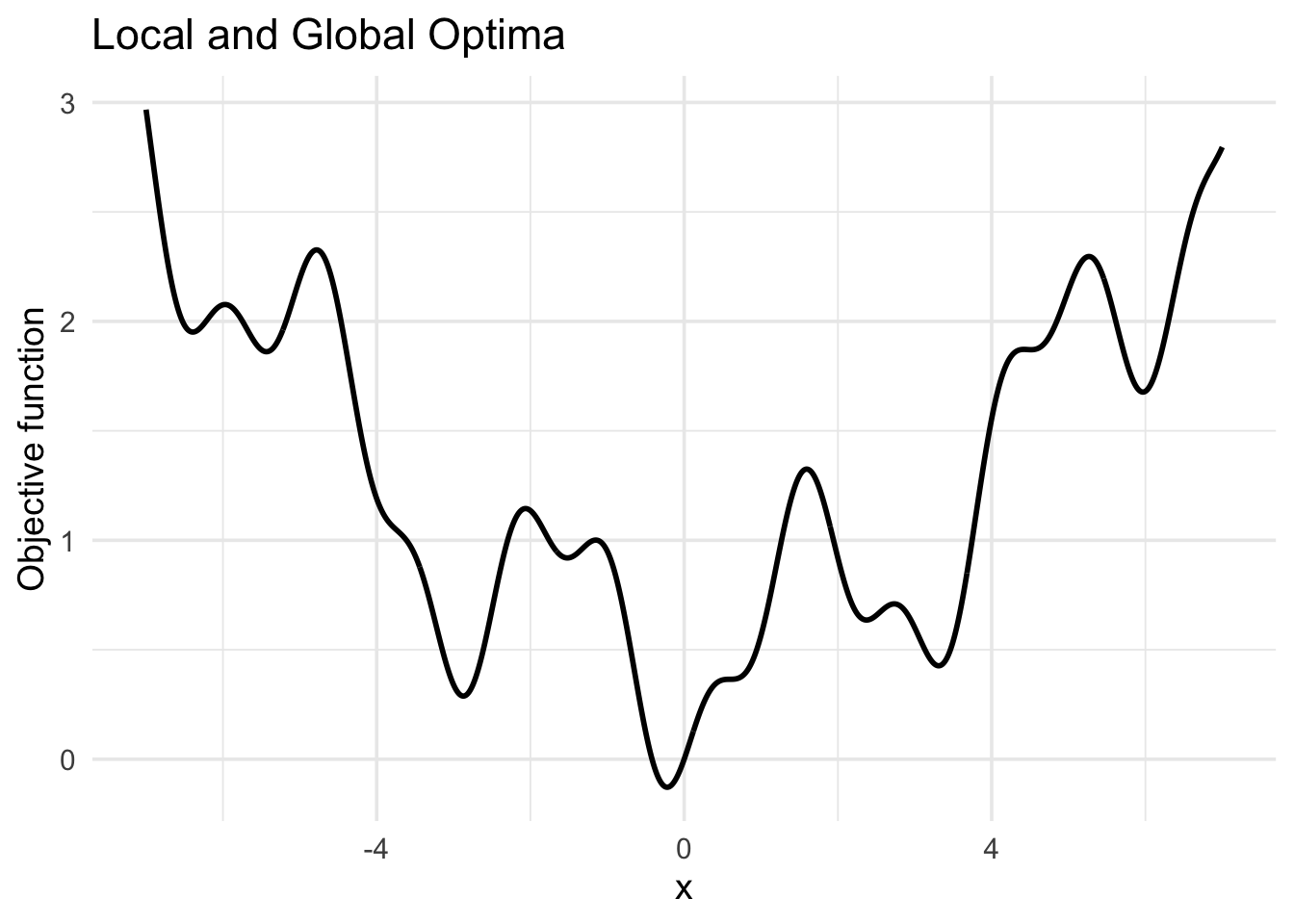
\[ Q(x) = 0.05x^2 + \sin^2(x) + 0.2\sin(5x). \]

Code
objective <- function(x) {
  0.05 * x^2 +
    sin(x)^2 +
    0.2 * sin(5 * x)
}

x_grid <- seq(
  -7,
  7,
  length.out = 1000
)

objective_data <- data.frame(
  x = x_grid,
  objective = objective(x_grid)
)

ggplot(
  objective_data,
  aes(
    x = x,
    y = objective
  )
) +
  geom_line(linewidth = 1) +
  labs(
    x = "x",
    y = "Objective function",
    title = "Local and Global Optima"
  )

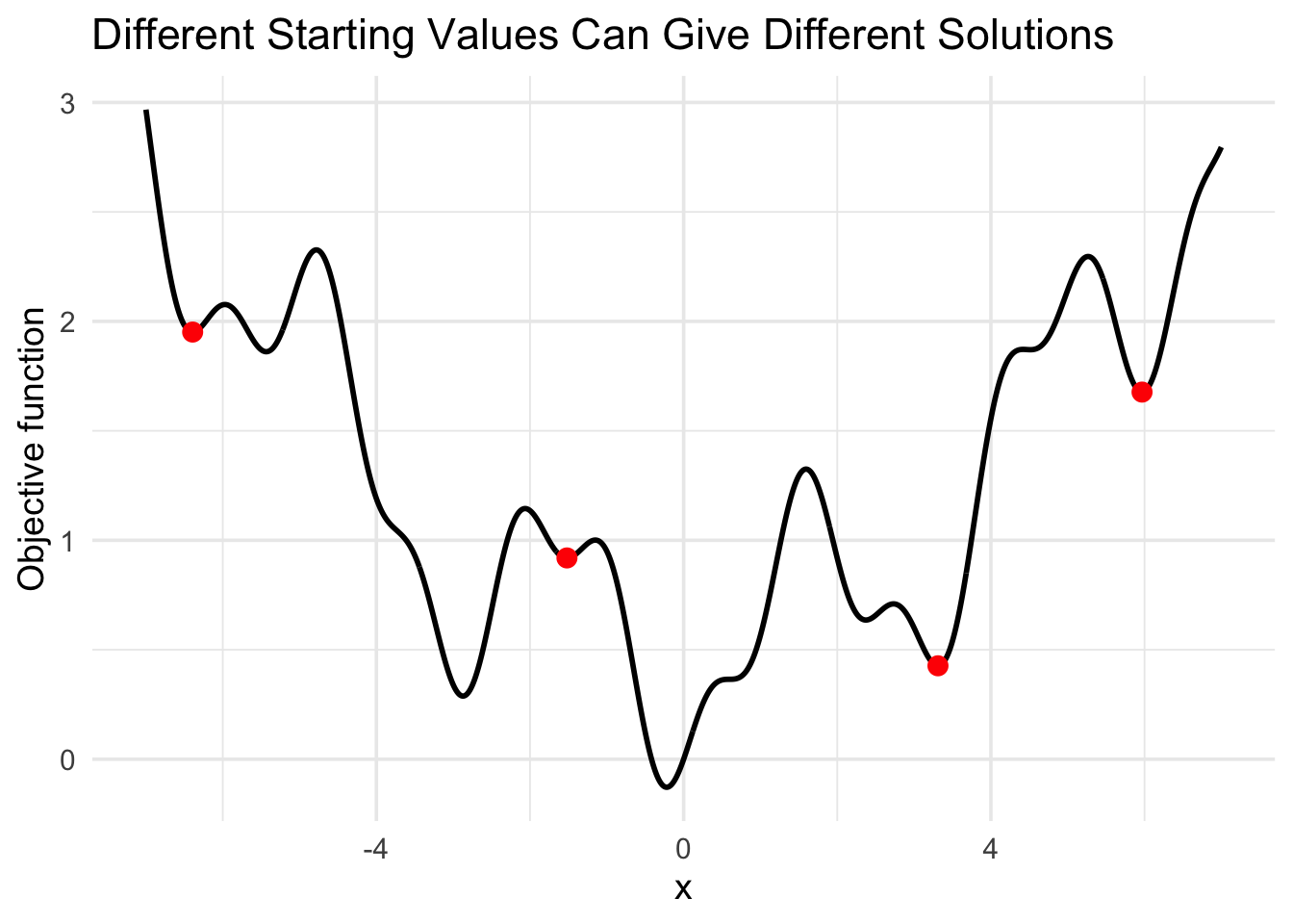
The objective contains several local minima.

A deterministic local optimizer may converge to different solutions depending on its starting value.

Code
starts <- c(
  -6,
  -2,
  2,
  6
)

solutions <- vapply(
  starts,
  function(x0) {
    optim(
      par = x0,
      fn = objective,
      method = "BFGS"
    )$par
  },
  numeric(1)
)

local_results <- data.frame(
  start = starts,
  solution = solutions,
  objective = objective(solutions)
)

local_results
  start  solution objective
1    -6 -6.392105 1.9511520
2    -2 -1.519268 0.9193572
3     2  3.310780 0.4266970
4     6  5.967669 1.6769489
Code
ggplot(
  objective_data,
  aes(
    x = x,
    y = objective
  )
) +
  geom_line(linewidth = 1) +
  geom_point(
    data = local_results,
    col = "red",
    aes(
      x = solution,
      y = objective
    ),
    size = 3
  ) +
  labs(
    x = "x",
    y = "Objective function",
    title = "Different Starting Values Can Give Different Solutions"
  )

If the algorithm is deterministic, why can different starting values still produce different answers?

The important distinction is

\[ \boxed{ \text{Local Optimum} \neq \text{Global Optimum}. } \]

3.5 Deterministic Numerical Methods

We first study several deterministic numerical methods.

3.5.1 Root Finding

Root finding solves

\[ f(x)=0. \]

Why is root finding relevant to optimization?

If \(Q(x)\) is differentiable and \(x^*\) is an interior optimum, then typically

\[ Q'(x^*)=0. \]

Therefore, optimization can sometimes be converted into

\[ f(x) = Q'(x) = 0. \]

A root of \(Q'(x)\) is only a candidate optimum. It may correspond to a minimum, maximum, or another stationary point.

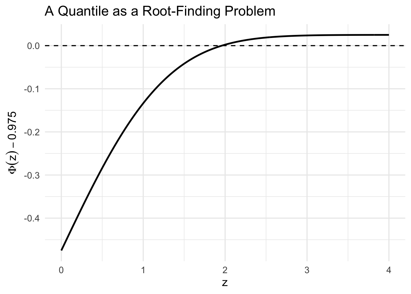
Suppose we want the 97.5th percentile of a standard normal distribution.

We seek \(z\) such that

\[ P(Z\le z) = 0.975. \]

Equivalently,

\[ \Phi(z)-0.975=0. \]

Code
f_root <- function(z) {
  pnorm(z) - 0.975
}

z_grid <- seq(
  0,
  4,
  length.out = 400
)

root_data <- data.frame(
  z = z_grid,
  f = f_root(z_grid)
)

ggplot(
  root_data,
  aes(
    x = z,
    y = f
  )
) +
  geom_line(linewidth = 1) +
  geom_hline(
    yintercept = 0,
    linetype = "dashed"
  ) +
  labs(
    x = "z",
    y = expression(Phi(z) - 0.975),
    title = "A Quantile as a Root-Finding Problem"
  )

R can solve the root directly:

Code
root_R <- uniroot(
  f_root,
  interval = c(0, 4)
)$root

c(
  root_finding = root_R,
  qnorm = qnorm(0.975)
)
root_finding        qnorm 
    1.959963     1.959964 

Thus,

\[ \boxed{ \text{Quantile Calculation} \Longleftrightarrow \text{Root Finding}. } \]

Why do uniroot() and qnorm() give essentially the same answer?

3.5.2 Bisection Method

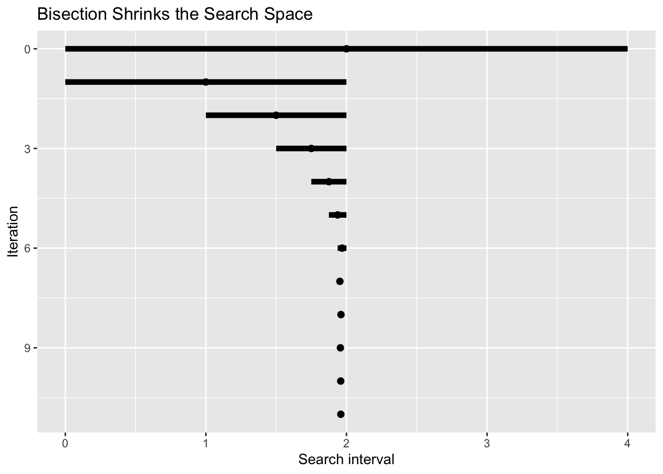
The bisection method is similar to a binary search.

Suppose \(f\) is continuous and

\[ f(a)f(b)<0. \]

Then there must be at least one root between \(a\) and \(b\).

  1. Choose \(a\) and \(b\) such that \(f(a)f(b)<0\).

  2. Compute

\[ c=\frac{a+b}{2}. \]

  1. Keep the half containing the sign change.

  2. Repeat until the interval is sufficiently small.

The main intuition is

\[ \boxed{ \text{Each iteration cuts the search interval approximately in half}. } \]

Code
bisect_trace <- function(
    f,
    a,
    b,
    tol = 1e-6,
    maxit = 100
) {

  if (f(a) * f(b) > 0) {
    stop("f(a) and f(b) must have opposite signs.")
  }

  history <- data.frame()

  for (k in 0:maxit) {

    midpoint <- (a + b) / 2

    history <- rbind(
      history,
      data.frame(
        iteration = k,
        a = a,
        b = b,
        midpoint = midpoint,
        f_midpoint = f(midpoint)
      )
    )

    if (
      abs(f(midpoint)) < tol ||
      (b - a) / 2 < tol
    ) {
      break
    }

    if (f(a) * f(midpoint) <= 0) {
      b <- midpoint
    } else {
      a <- midpoint
    }
  }

  history
}

bisect_history <- bisect_trace(
  f_root,
  a = 0,
  b = 4
)

tail(bisect_history)
   iteration        a        b midpoint    f_midpoint
7          6 1.937500 2.000000 1.968750  5.090967e-04
8          7 1.937500 1.968750 1.953125 -4.023926e-04
9          8 1.953125 1.968750 1.960938  5.684292e-05
10         9 1.953125 1.960938 1.957031 -1.718972e-04
11        10 1.957031 1.960938 1.958984 -5.730834e-05
12        11 1.958984 1.960938 1.959961 -1.780850e-07

Visualizing

Code
ggplot(
  bisect_history,
  aes(y = iteration)
) +
  geom_segment(
    aes(
      x = a,
      xend = b,
      yend = iteration
    ),
    linewidth = 2
  ) +
  geom_point(
    aes(x = midpoint),
    size = 2
  ) +
  scale_y_reverse() +
  labs(
    x = "Search interval",
    y = "Iteration",
    title = "Bisection Shrinks the Search Space"
  )

Bisection requires continuity and a sign change, but does not require derivatives.

What information does bisection use about the function?

What information does it ignore?

3.5.3 Newton-Raphson Method

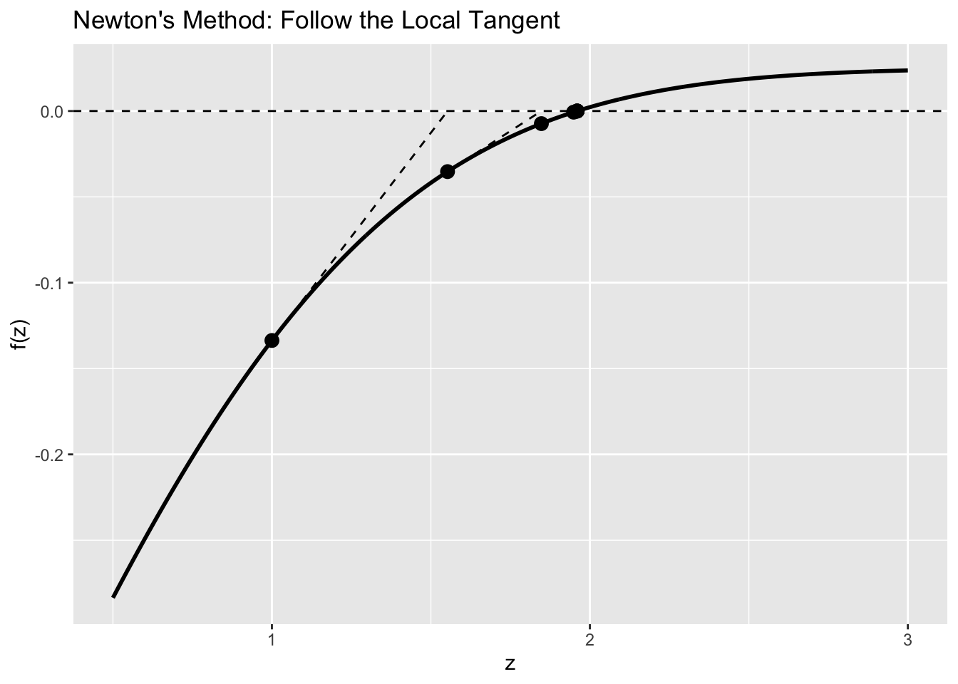
Newton’s method uses local derivative information.

Around the current estimate \(x_k\),

\[ f(x) \approx f(x_k) + f'(x_k)(x-x_k). \]

Set the approximation equal to zero:

\[ 0 = f(x_k) + f'(x_k)(x_{k+1}-x_k). \]

Therefore,

\[ \boxed{ x_{k+1} = x_k - \frac{f(x_k)} {f'(x_k)} }. \]

The intuition is:

Approximate the function locally by a straight line and use the root of that line as the next guess.

For

\[ f(z) = \Phi(z)-0.975, \]

we have

\[ f'(z) = \phi(z). \]

Code
f <- function(z) {
  pnorm(z) - 0.975
}

df <- function(z) {
  dnorm(z)
}
Code
newton_trace <- function(
    f,
    df,
    x0,
    tol = 1e-8,
    maxit = 100
) {

  x <- x0

  history <- data.frame(
    iteration = 0,
    x = x,
    fx = f(x)
  )

  for (k in seq_len(maxit)) {

    dfx <- df(x)

    if (abs(dfx) < 1e-12) {
      stop("Derivative is too close to zero.")
    }

    x_new <- x - f(x) / dfx

    history <- rbind(
      history,
      data.frame(
        iteration = k,
        x = x_new,
        fx = f(x_new)
      )
    )

    if (abs(x_new - x) < tol) {
      break
    }

    x <- x_new
  }

  history
}

newton_history <- newton_trace(
  f,
  df,
  x0 = 1
)

newton_history
  iteration        x            fx
1         0 1.000000 -1.336553e-01
2         1 1.552361 -3.528790e-02
3         2 1.847484 -7.338509e-03
4         3 1.948843 -6.570601e-04
5         4 1.959844 -7.006182e-06
6         5 1.959964 -8.227717e-10
7         6 1.959964  0.000000e+00
8         7 1.959964  0.000000e+00

3.5.4 Visualizing Newton’s Method

Code
tangent_data <- data.frame(
  x = head(newton_history$x, -1),
  y = head(newton_history$fx, -1),
  xend = tail(newton_history$x, -1),
  yend = 0
)

z_grid <- seq(
  0.5,
  3,
  length.out = 400
)

newton_function_data <- data.frame(
  z = z_grid,
  f = f(z_grid)
)

ggplot(
  newton_function_data,
  aes(
    x = z,
    y = f
  )
) +
  geom_line(linewidth = 1) +
  geom_hline(
    yintercept = 0,
    linetype = "dashed"
  ) +
  geom_segment(
    data = tangent_data,
    aes(
      x = x,
      y = y,
      xend = xend,
      yend = yend
    ),
    inherit.aes = FALSE,
    linetype = "dashed"
  ) +
  geom_point(
    data = newton_history,
    aes(
      x = x,
      y = fx
    ),
    inherit.aes = FALSE,
    size = 3
  ) +
  labs(
    x = "z",
    y = "f(z)",
    title = "Newton's Method: Follow the Local Tangent"
  )

Newton’s method can converge very quickly near the root.

However, if

\[ f'(x_k)\approx0, \]

then the update may become very large and unstable.

What happens to Newton’s update when \(f'(x_k)\) is close to zero?

3.5.5 Secant Method

Newton’s method requires the derivative \(f'(x)\).

If the derivative is unavailable or expensive, we can approximate it using two previous points:

\[ f'(x_k) \approx \frac{ f(x_k)-f(x_{k-1}) }{ x_k-x_{k-1} }. \]

Substituting this into Newton’s update gives

\[ \boxed{ x_{k+1} = x_k - f(x_k) \frac{ x_k-x_{k-1} }{ f(x_k)-f(x_{k-1}) } }. \]

Code
secant_trace <- function(
    f,
    x0,
    x1,
    tol = 1e-8,
    maxit = 100
) {

  history <- data.frame(
    iteration = c(0, 1),
    x = c(x0, x1),
    fx = c(
      f(x0),
      f(x1)
    )
  )

  for (k in 2:maxit) {

    f0 <- f(x0)
    f1 <- f(x1)

    denominator <- f1 - f0

    if (abs(denominator) < 1e-12) {
      stop("Secant denominator is too close to zero.")
    }

    x2 <- x1 -
      f1 * (x1 - x0) /
      denominator

    history <- rbind(
      history,
      data.frame(
        iteration = k,
        x = x2,
        fx = f(x2)
      )
    )

    if (abs(x2 - x1) < tol) {
      break
    }

    x0 <- x1
    x1 <- x2
  }

  history
}

secant_history <- secant_trace(
  f,
  x0 = 1,
  x1 = 2.5
)

secant_history
   iteration        x            fx
1          0 1.000000 -1.336553e-01
2          1 2.500000  1.879033e-02
3          2 2.315111  1.469657e-02
4          3 1.651361 -2.433241e-02
5          4 2.065173  5.546662e-03
6          5 1.988354  1.613717e-03
7          6 1.956835 -1.834592e-04
8          7 1.960052  5.151979e-06
9          8 1.959964  1.577731e-08
10         9 1.959964 -1.363021e-12
11        10 1.959964  0.000000e+00

The three methods illustrate different computational trade-offs.

Method Derivative? Starting information Main advantage Main limitation
Bisection No \([a,b]\) Very reliable Slower
Newton Yes \(x_0\) Very fast near root Can fail
Secant No \(x_0,x_1\) Fast without derivative Less reliable

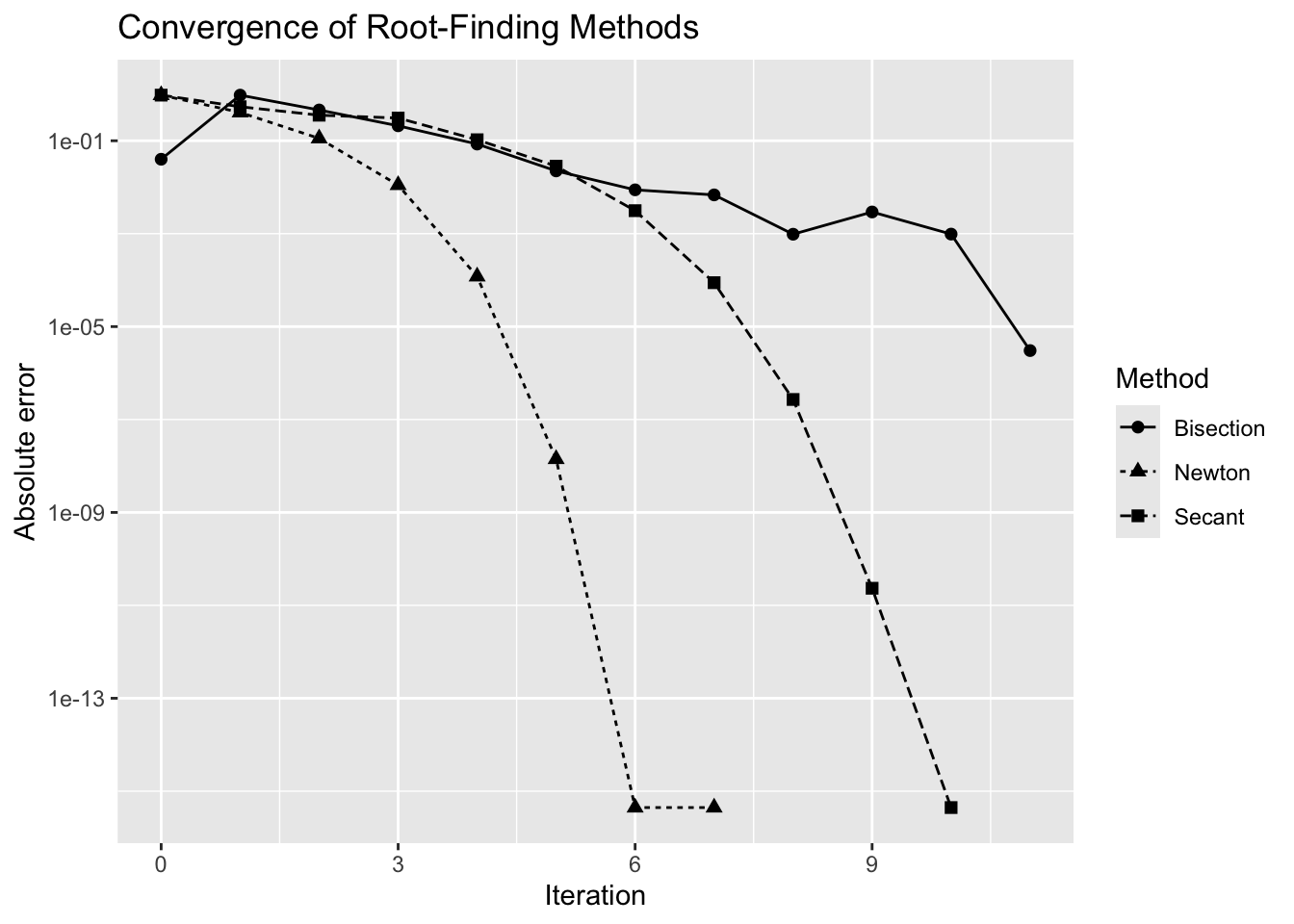
3.6 Convergence

Suppose an iterative algorithm produces

\[ x_0,x_1,x_2,\ldots \]

and converges to a solution \(x^*\).

Define

\[ e_k = |x_k-x^*|. \]

A common description of convergence is

\[ e_{k+1} \approx C e_k^q. \]

The value \(q\) describes how quickly the error decreases.

  • Linear convergence: \(q=1\).
  • Superlinear convergence: faster than linear.
  • Quadratic convergence: \(q=2\).

Under suitable conditions:

  • bisection converges linearly;
  • the secant method converges superlinearly;
  • Newton’s method converges quadratically near the root.

3.6.1 Comparing Convergence in R

Code
true_root <- qnorm(0.975)

bisection_error <- data.frame(
  iteration = bisect_history$iteration,
  error = abs(
    bisect_history$midpoint -
      true_root
  ),
  method = "Bisection"
)

newton_error <- data.frame(
  iteration = newton_history$iteration,
  error = abs(
    newton_history$x -
      true_root
  ),
  method = "Newton"
)

secant_error <- data.frame(
  iteration = secant_history$iteration,
  error = abs(
    secant_history$x -
      true_root
  ),
  method = "Secant"
)

convergence_data <- rbind(
  bisection_error,
  newton_error,
  secant_error
)

convergence_data <- subset(
  convergence_data,
  error > .Machine$double.eps
)
Code
ggplot(
  convergence_data,
  aes(
    x = iteration,
    y = error,
    linetype = method,
    shape = method
  )
) +
  geom_line() +
  geom_point(size = 2) +
  scale_y_log10() +
  labs(
    x = "Iteration",
    y = "Absolute error",
    title = "Convergence of Root-Finding Methods",
    linetype = "Method",
    shape = "Method"
  )

Which method appears to converge fastest?

Does fewer iterations necessarily mean less computation?

A useful computational perspective is

\[ \boxed{ \text{Total Computational Cost} \approx \text{Cost per Iteration} \times \text{Number of Iterations}. } \]

3.7 From One Dimension to Multiple Dimensions

Most statistical problems involve more than one parameter.

Instead of

\[ x\in\mathbb R, \]

we now consider

\[ \boldsymbol{\theta} = (\theta_1,\ldots,\theta_p)^\top \in \mathbb R^p. \]

The one-dimensional concepts generalize naturally:

\[ Q'(x) \quad\Longrightarrow\quad \nabla Q(\boldsymbol{\theta}), \]

and

\[ Q''(x) \quad\Longrightarrow\quad H(\boldsymbol{\theta}). \]

The gradient is

\[ \nabla Q(\boldsymbol{\theta}) = \begin{pmatrix} \partial Q/\partial\theta_1\\ \vdots\\ \partial Q/\partial\theta_p \end{pmatrix}, \]

and the Hessian is the matrix of second derivatives,

\[ H(\boldsymbol{\theta}) = \left[ \frac{ \partial^2 Q }{ \partial\theta_j\partial\theta_k } \right]. \]

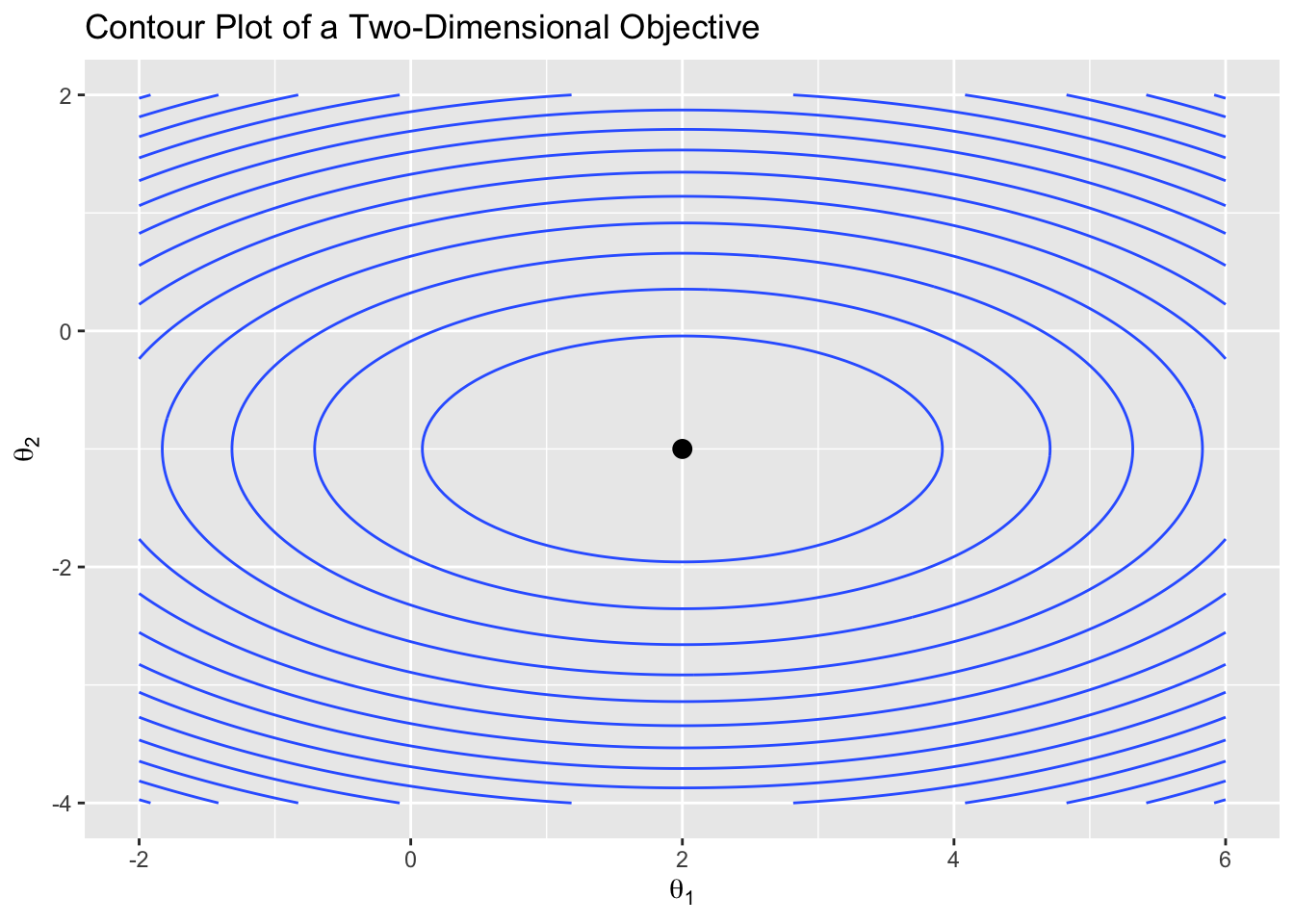
Consider

\[ Q(\theta_1,\theta_2) = (\theta_1-2)^2 + 4(\theta_2+1)^2. \]

Code
objective_2d <- function(theta1, theta2) {
  (theta1 - 2)^2 +
    4 * (theta2 + 1)^2
}

theta1_grid <- seq(
  -2,
  6,
  length.out = 150
)

theta2_grid <- seq(
  -4,
  2,
  length.out = 150
)

objective_grid <- expand.grid(
  theta1 = theta1_grid,
  theta2 = theta2_grid
)

objective_grid$value <- with(
  objective_grid,
  objective_2d(theta1, theta2)
)

ggplot(
  objective_grid,
  aes(
    x = theta1,
    y = theta2,
    z = value
  )
) +
  geom_contour(
    bins = 15
  ) +
  geom_point(
    data = data.frame(
      theta1 = 2,
      theta2 = -1
    ),
    aes(
      x = theta1,
      y = theta2
    ),
    inherit.aes = FALSE,
    size = 3
  ) +
  labs(
    x = expression(theta[1]),
    y = expression(theta[2]),
    title = "Contour Plot of a Two-Dimensional Objective"
  )

The minimum occurs at

\[ \boldsymbol{\theta}^* = \begin{pmatrix} 2\\ -1 \end{pmatrix}. \]

3.8 Gradient Descent

The gradient points in the direction of greatest increase.

Therefore,

\[ -\nabla Q(\boldsymbol{\theta}) \]

is a natural direction for decreasing the objective.

Gradient descent updates

\[ \boxed{ \boldsymbol{\theta}_{k+1} = \boldsymbol{\theta}_k - \alpha_k \nabla Q(\boldsymbol{\theta}_k), } \]

where \(\alpha_k>0\) is the step size or learning rate.

For the quadratic example,

\[ \nabla Q(\theta_1,\theta_2) = \begin{pmatrix} 2(\theta_1-2)\\ 8(\theta_2+1) \end{pmatrix}. \]

Code
gradient_2d <- function(theta) {
  c(
    2 * (theta[1] - 2),
    8 * (theta[2] + 1)
  )
}

gradient_descent <- function(
    start,
    alpha = 0.1,
    maxit = 30
) {

  theta <- start

  history <- data.frame(
    iteration = 0,
    theta1 = theta[1],
    theta2 = theta[2]
  )

  for (k in seq_len(maxit)) {

    theta <-
      theta -
      alpha * gradient_2d(theta)

    history <- rbind(
      history,
      data.frame(
        iteration = k,
        theta1 = theta[1],
        theta2 = theta[2]
      )
    )
  }

  history
}

gd_path <- gradient_descent(
  start = c(-1, 1),
  alpha = 0.1,
  maxit = 20
)

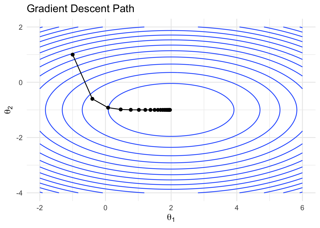
3.8.1 Visualizing the Optimization Path

Code
ggplot(
  objective_grid,
  aes(
    x = theta1,
    y = theta2,
    z = value
  )
) +
  geom_contour(
    bins = 15
  ) +
  geom_path(
    data = gd_path,
    aes(
      x = theta1,
      y = theta2
    ),
    inherit.aes = FALSE
  ) +
  geom_point(
    data = gd_path,
    aes(
      x = theta1,
      y = theta2
    ),
    inherit.aes = FALSE,
    size = 2
  ) +
  labs(
    x = expression(theta[1]),
    y = expression(theta[2]),
    title = "Gradient Descent Path"
  )

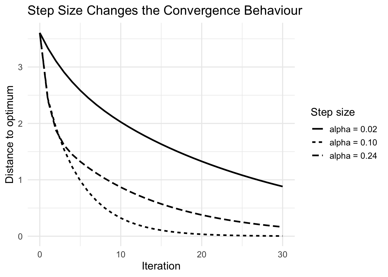
What happens if the step size \(\alpha\) is too small?

What happens if it is too large?

3.8.2 Step Size Matters

Code
gd_small <- gradient_descent(
  start = c(-1, 1),
  alpha = 0.02,
  maxit = 30
)

gd_medium <- gradient_descent(
  start = c(-1, 1),
  alpha = 0.1,
  maxit = 30
)

gd_large <- gradient_descent(
  start = c(-1, 1),
  alpha = 0.24,
  maxit = 30
)

gd_compare <- rbind(
  transform(
    gd_small,
    step = "alpha = 0.02"
  ),
  transform(
    gd_medium,
    step = "alpha = 0.10"
  ),
  transform(
    gd_large,
    step = "alpha = 0.24"
  )
)

gd_compare$error <-
  sqrt(
    (gd_compare$theta1 - 2)^2 +
      (gd_compare$theta2 + 1)^2
  )

ggplot(
  gd_compare,
  aes(
    x = iteration,
    y = error,
    linetype = step
  )
) +
  geom_line(linewidth = 1) +
  labs(
    x = "Iteration",
    y = "Distance to optimum",
    linetype = "Step size",
    title = "Step Size Changes the Convergence Behaviour"
  )

3.9 Multivariate Newton’s Method

In one dimension,

\[ x_{k+1} = x_k - \frac{Q'(x_k)}{Q''(x_k)}. \]

In multiple dimensions, this becomes

\[ \boxed{ \boldsymbol{\theta}_{k+1} = \boldsymbol{\theta}_k - H(\boldsymbol{\theta}_k)^{-1} \nabla Q(\boldsymbol{\theta}_k). } \]

However, computationally we usually do not calculate the inverse explicitly.

Instead, solve

\[ H(\boldsymbol{\theta}_k) \boldsymbol{d}_k = -\nabla Q(\boldsymbol{\theta}_k), \]

and update

\[ \boldsymbol{\theta}_{k+1} = \boldsymbol{\theta}_k + \boldsymbol{d}_k. \]

Why do we solve a linear system instead of explicitly computing

\[ H^{-1}? \]

This connects directly to the earlier discussion of numerical stability and matrix inversion.

3.10 Quasi-Newton Methods

Newton’s method requires the Hessian.

For high-dimensional statistical models, computing the Hessian can be expensive.

Quasi-Newton methods approximate curvature information rather than calculating the Hessian directly.

One of the most widely used methods is BFGS.

In R:

optim(
  par = start,
  fn = objective,
  method = "BFGS"
)

The main computational idea is

\[ \boxed{ \text{Use curvature information} \quad\text{without repeatedly computing the full Hessian}. } \]

Consider

\[ Y_i \sim \operatorname{Bernoulli}(p_i), \]

with

\[ \log \left( \frac{p_i}{1-p_i} \right) = \beta_0+\beta_1x_i. \]

The parameter is now a vector

\[ \boldsymbol{\beta} = (\beta_0,\beta_1)^\top. \]

There is no closed-form MLE, so logistic regression requires numerical optimization.

Code
set.seed(8670)

n <- 200

x_logit <- rnorm(n)

beta_true <- c(
  -0.5,
  1.5
)

eta <-
  beta_true[1] +
  beta_true[2] * x_logit

p <- plogis(eta)

y_logit <- rbinom(
  n,
  size = 1,
  prob = p
)

Define the negative log-likelihood:

Code
logistic_nll <- function(beta) {

  eta <-
    beta[1] +
    beta[2] * x_logit

  p <- plogis(eta)

  -sum(
    dbinom(
      y_logit,
      size = 1,
      prob = p,
      log = TRUE
    )
  )
}

Estimate the coefficients using BFGS:

Code
fit_optim <- optim(
  par = c(0, 0),
  fn = logistic_nll,
  method = "BFGS"
)

fit_optim$par
[1] -0.381730  1.014505

Compare with glm():

Code
fit_glm <- glm(
  y_logit ~ x_logit,
  family = binomial()
)

coef(fit_glm)
(Intercept)     x_logit 
 -0.3817297   1.0145052 
Code
fit_optim$par
[1] -0.381730  1.014505

Why is comparing optim() with glm() useful?

This illustrates the complete computational-statistics workflow:

\[ \boxed{ \text{Statistical Model} \rightarrow \text{Likelihood} \rightarrow \text{Optimization} \rightarrow \text{Algorithm} \rightarrow \text{Validation}. } \]

3.11 Scaling and Conditioning

Optimization can behave very differently when parameters operate on different scales.

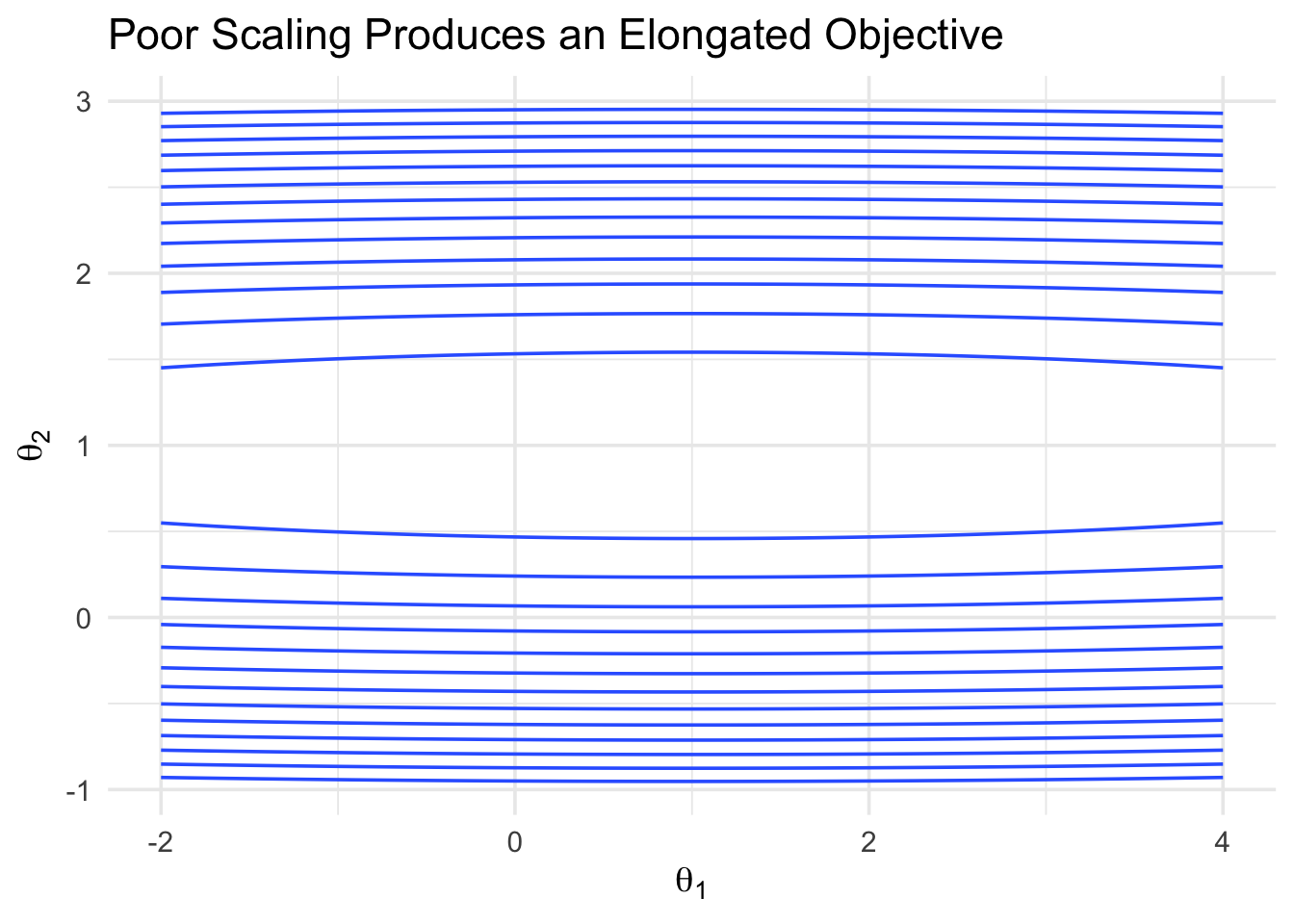
Consider

\[ Q(\theta_1,\theta_2) = (\theta_1-1)^2 + 100(\theta_2-1)^2. \]

Code
scaled_objective <- function(theta1, theta2) {
  (theta1 - 1)^2 +
    100 * (theta2 - 1)^2
}

scale_grid <- expand.grid(
  theta1 = seq(
    -2,
    4,
    length.out = 150
  ),
  theta2 = seq(
    -1,
    3,
    length.out = 150
  )
)

scale_grid$value <- with(
  scale_grid,
  scaled_objective(
    theta1,
    theta2
  )
)

ggplot(
  scale_grid,
  aes(
    x = theta1,
    y = theta2,
    z = value
  )
) +
  geom_contour(
    bins = 15
  ) +
  labs(
    x = expression(theta[1]),
    y = expression(theta[2]),
    title = "Poor Scaling Produces an Elongated Objective"
  )

A highly elongated objective can cause gradient-based algorithms to zig-zag and converge slowly.

This illustrates another important principle:

\[ \boxed{ \text{Same mathematical problem} + \text{different scaling} \Longrightarrow \text{different computational behaviour}. } \]

3.12 Metaheuristic Methods

Deterministic optimization methods can work extremely well for smooth and well-behaved objectives.

However, they may struggle when the objective:

  • contains many local optima;
  • is not differentiable;
  • is discontinuous;
  • has a complicated search space.

Metaheuristic methods use broader stochastic exploration.

The key idea is

\[ \boxed{ \text{Explore broadly} \quad\longrightarrow\quad \text{search more locally later}. } \]

Why Accept a Worse Solution?

A local deterministic method usually attempts to improve the objective at every step.

A stochastic method may deliberately accept a worse solution.

Why would an optimization algorithm ever accept a worse solution?

Temporarily moving to a worse location can allow the algorithm to escape a local optimum and later reach a better region.

3.13 Simulated Annealing

Simulated annealing is a stochastic optimization method inspired by the physical process of heating and slowly cooling a material.

Suppose the current solution is \(x_k\) and a candidate solution \(x'\) is generated.

For a minimization problem, if

\[ Q(x')<Q(x_k), \]

the new solution is accepted.

If

\[ Q(x')>Q(x_k), \]

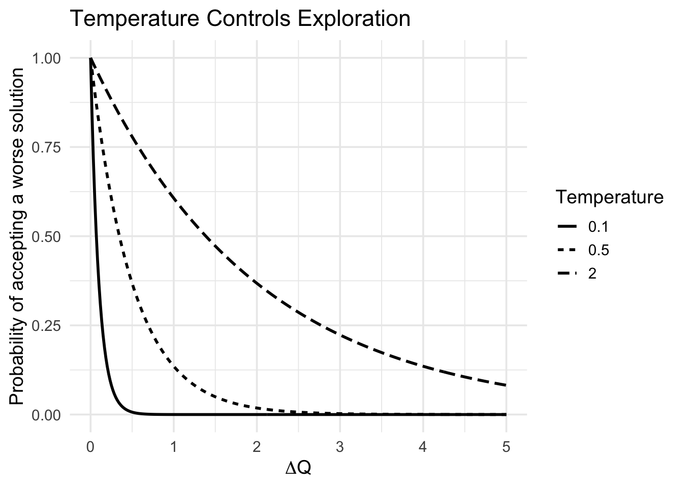
the worse solution may still be accepted with probability

\[ \boxed{ P(\text{accept}) = \exp \left( -\frac{\Delta Q}{T} \right), } \]

where

\[ \Delta Q = Q(x')-Q(x_k)>0. \]

The parameter \(T\) is called the temperature.

When

\[ T \quad\text{is large}, \]

the algorithm explores more broadly.

When

\[ T \quad\text{is small}, \]

the algorithm becomes more selective.

Visualizing the Acceptance Probability

Code
delta_grid <- seq(
  0,
  5,
  length.out = 300
)

temperature <- c(
  0.1,
  0.5,
  2
)

sa_probability <- expand.grid(
  delta = delta_grid,
  temperature = temperature
)

sa_probability$probability <-
  exp(
    -sa_probability$delta /
      sa_probability$temperature
  )

sa_probability$temperature <-
  factor(
    sa_probability$temperature
  )

ggplot(
  sa_probability,
  aes(
    x = delta,
    y = probability,
    linetype = temperature
  )
) +
  geom_line(linewidth = 1) +
  labs(
    x = expression(Delta * Q),
    y = "Probability of accepting a worse solution",
    linetype = "Temperature",
    title = "Temperature Controls Exploration"
  )

At high temperature, why is the algorithm more willing to accept a poor move?

What happens as the temperature approaches zero?

3.13.1 Simulated Annealing in R

R provides simulated annealing through

optim(
  ...,
  method = "SANN"
)

Using the earlier multimodal objective:

Code
set.seed(8670)

sa_fit <- optim(
  par = 5,
  fn = objective,
  method = "SANN",
  control = list(
    maxit = 3000
  )
)

sa_fit$par
[1] -0.1958383
Code
sa_fit$value
[1] -0.1262269

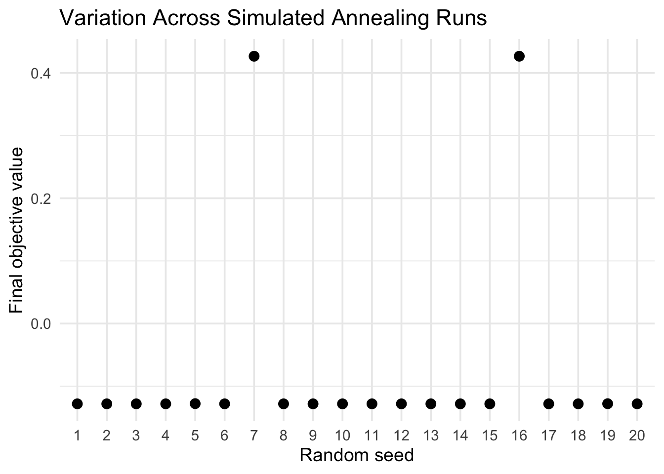
Because simulated annealing is stochastic, different seeds may produce different results.

Code
seeds <- 1:20

sa_solution <- vapply(
  seeds,
  function(seed) {

    set.seed(seed)

    optim(
      par = 5,
      fn = objective,
      method = "SANN",
      control = list(
        maxit = 3000
      )
    )$par

  },
  numeric(1)
)

sa_data <- data.frame(
  seed = seeds,
  solution = sa_solution,
  objective = objective(sa_solution)
)

ggplot(
  sa_data,
  aes(
    x = factor(seed),
    y = objective
  )
) +
  geom_point(size = 3) +
  labs(
    x = "Random seed",
    y = "Final objective value",
    title = "Variation Across Simulated Annealing Runs"
  )

Advantages of Simulated Annealing

  • Can escape local optima.
  • Does not require derivatives.
  • Easy to adapt to many objective functions.
  • Useful for multimodal problems.

Limitations of Simulated Annealing

  • Can require many function evaluations.
  • Results vary across runs.
  • Performance depends on the cooling schedule.
  • Does not guarantee the global optimum.

3.14 Genetic Algorithm

A genetic algorithm uses a population of candidate solutions rather than one current solution.

The basic cycle is

\[ \boxed{ \text{Selection} \rightarrow \text{Crossover} \rightarrow \text{Mutation} \rightarrow \text{New Generation}. } \]

3.14.1 Selection

Better candidate solutions are more likely to remain in the population.

3.14.2 Crossover

Information from two candidate solutions is combined to create new candidates.

3.14.3 Mutation

Random changes are introduced to preserve diversity and explore new regions.

The key difference from simulated annealing is:

\[ \boxed{ \text{SA: one evolving solution} \qquad \text{GA: a population of solutions}. } \]

Advantages

  • Explores several regions simultaneously.
  • Does not require gradients.
  • Flexible for continuous and discrete problems.

Limitations

  • Can require many objective evaluations.
  • Requires tuning of population size and mutation rate.
  • Can converge slowly.
  • Does not guarantee a global optimum.

3.15 Particle Swarm Optimization

Particle swarm optimization also maintains a population of candidate solutions called particles.

Each particle uses information about:

  • its current location;
  • its previous velocity;
  • its own best location;
  • the best location found by the group.

A simplified velocity update is

\[ v_{i,k+1} = w v_{i,k} + c_1r_1(p_i-x_{i,k}) + c_2r_2(g-x_{i,k}), \]

followed by

\[ x_{i,k+1} = x_{i,k} + v_{i,k+1}. \]

The intuition is

\[ \boxed{ \text{Momentum} + \text{Individual Experience} + \text{Group Experience} + \text{Randomness}. } \]

3.15.1 Advantages

  • Does not require derivatives.
  • Explores multiple regions simultaneously.
  • Relatively intuitive and flexible.

3.15.2 Limitations

  • May require many function evaluations.
  • Sensitive to tuning parameters.
  • Can converge prematurely.
  • Global optimality is not guaranteed.

3.16 Deterministic versus Metaheuristic Methods

The two families search very differently.

Method Type Derivatives Search Main Advantage Main Limitation
Bisection Deterministic No Root finding Very reliable Slow
Newton Deterministic Yes Local Very fast near solution Sensitive to derivative and start
Secant Deterministic No Local Fast without derivative Less reliable
Gradient Descent Deterministic Gradient Local Simple and scalable Step size matters
BFGS Deterministic Usually gradient Local Efficient for smooth problems Can reach local optimum
Simulated Annealing Metaheuristic No Global exploration Can escape local optima Slow and stochastic
Genetic Algorithm Metaheuristic No Population Flexible search Computationally expensive
Particle Swarm Metaheuristic No Population Cooperative exploration Requires tuning

The important question is not

Which algorithm is the best?

Instead, ask

Which algorithm is appropriate for the structure of the statistical problem?

For a smooth and well-behaved objective,

\[ \text{deterministic methods} \]

are usually preferable.

For a highly multimodal, irregular, or derivative-free objective,

\[ \text{metaheuristic methods} \]

may become useful.

Suppose the objective is smooth, convex, and easy to differentiate.

Would you choose BFGS or simulated annealing?

What changes if the objective has many local minima and no useful derivatives?

3.17 Computational Perspective

The goal is not simply to memorize optimization algorithms.

For a statistical problem, ask:

  1. What is the statistical quantity we want?
  2. Can it be written as an optimization or root-finding problem?
  3. Is there a closed-form solution?
  4. Is the parameter scalar or multivariate?
  5. Is the objective smooth?
  6. Are derivatives available?
  7. Are there many local optima?
  8. How sensitive is the method to the starting value?
  9. Is the computation numerically stable?
  10. How can we validate the result?

This brings us back to the central idea of statistical computing:

\[ \boxed{ \text{Theory} \Longleftrightarrow \text{Computation} \Longleftrightarrow \text{Practice}. } \]

3.18 Questions to Think at Home

  1. Why can a mathematically correct optimization formula still lead to a poor computational implementation?

  2. Why is a closed-form solution useful even when numerical optimization will eventually be used?

  3. Why is bisection more reliable than Newton’s method, and what is the computational cost of that reliability?

  4. What additional information does Newton’s method use compared with bisection?

  5. Why can different starting values lead to different solutions for the same objective function?

  6. What role does the step size play in gradient descent?

  7. Why might poor scaling make optimization difficult?

  8. Why is solving

\[ H\boldsymbol{d} = -\nabla Q \]

usually preferable to explicitly computing \(H^{-1}\)?

  1. Why can BFGS be useful when the Hessian is expensive to compute?

  2. Why might a metaheuristic algorithm deliberately accept a worse solution?

  3. When would you prefer simulated annealing over a deterministic local optimizer?

  4. What is the main difference between simulated annealing, genetic algorithms, and particle swarm optimization?

  5. Why does fewer iterations not necessarily imply lower computational cost?

  6. How are optimization, likelihood estimation, and statistical inference connected?

3.19 Takeaways

  • Many statistical estimators are solutions to optimization problems.
  • Closed-form solutions are convenient but often unavailable.
  • Numerical optimization connects statistical theory with practical computation.
  • Root finding is closely related to optimization.
  • Bisection is reliable but relatively slow.
  • Newton’s method is fast near a solution but uses derivative information.
  • The secant method approximates derivative information numerically.
  • Multivariate optimization replaces derivatives with gradients and Hessians.
  • Gradient descent uses local first-order information.
  • Newton’s method uses curvature information through the Hessian.
  • BFGS approximates curvature without repeatedly computing the full Hessian.
  • Scaling can strongly affect computational performance.
  • Deterministic methods are usually efficient for smooth, well-behaved objectives.
  • Metaheuristic methods trade speed and predictability for broader exploration.
  • Simulated annealing can escape local optima by occasionally accepting worse solutions.
  • Genetic algorithms and particle swarm optimization use populations of candidate solutions.
  • There is no universally best optimization algorithm.
  • A good computational method balances accuracy, stability, speed, and exploration.

3.20 Optimal topic: Real-World Applications

The applications in this chapter illustrate two uses of optimization: estimating unknown parameters from data and choosing an action under practical constraints. We will connect these ideas to drug development, investment portfolios, factory scheduling, and advertising budgets. The examples use simplified models of these real applications.

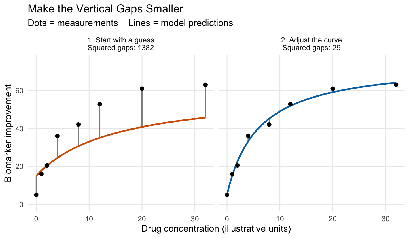
The situation. A research team measures drug concentration and the improvement in a biomarker. At low concentrations, more drug may produce a much larger response. At high concentrations, the response may level off. The team wants a curve that describes this pattern.

The computer’s job: adjust the curve until its predictions are close to the observed dots. The following measurements are invented for illustration.

Code
bio_data <- data.frame(Concentration = c(0, 1, 2, 4, 8, 12, 20, 32))
bio_data$Response <- 5 + 70 * bio_data$Concentration /
  (6 + bio_data$Concentration) + c(0, 1, -2, 3, -3, 1, 2, -1)

# Log parameters keep Emax and EC50 positive during the search.
bio_curve <- function(theta, concentration) {
  theta[1] + exp(theta[2]) * concentration /
    (exp(theta[3]) + concentration)
}
bio_error <- function(theta) {
  sum((bio_data$Response - bio_curve(theta, bio_data$Concentration))^2)
}
bio_start <- c(15, log(45), log(15))
bio_fit <- optim(
  bio_start, bio_error, method = "BFGS",
  control = list(maxit = 2000, reltol = 1e-12)
)
bio_stages <- c("1. Start with a guess\nSquared gaps: 1382",
                "2. Adjust the curve\nSquared gaps: 29")
bio_lines <- do.call(rbind, lapply(1:2, function(i) {
  concentration <- seq(0, 32, length.out = 250)
  theta <- if (i == 1) bio_start else bio_fit$par
  data.frame(Concentration = concentration,
             Response = bio_curve(theta, concentration),
             Stage = bio_stages[i])
}))
bio_points <- do.call(rbind, lapply(1:2, function(i) {
  theta <- if (i == 1) bio_start else bio_fit$par
  transform(bio_data, Predicted = bio_curve(theta, Concentration),
            Stage = bio_stages[i])
}))
ggplot(bio_lines, aes(Concentration, Response)) +
  geom_segment(
    data = bio_points,
    aes(xend = Concentration, yend = Predicted),
    colour = "grey55", linewidth = 0.7
  ) +
  geom_line(aes(colour = Stage), linewidth = 1) +
  geom_point(data = bio_points, size = 2) +
  facet_wrap(~Stage, nrow = 1) +
  scale_colour_manual(values = c("#D55E00", "#0072B2")) +
  scale_y_continuous(limits = c(0, 75)) +
  labs(x = "Drug concentration (illustrative units)",
       y = "Biomarker improvement",
       title = "Make the Vertical Gaps Smaller",
       subtitle = "Dots = measurements    Lines = model predictions") +
  theme_minimal(base_size = 12) +
  theme(legend.position = "none", panel.grid.minor = element_blank())
Two panels share the same measured dots. An initial orange curve lies far from most dots. The fitted blue curve follows the dots closely, leaving much smaller vertical prediction errors.
Figure 3.1: The same illustrative measurements, before and after fitting. Vertical gaps show prediction errors. Optimization reduces the sum of their squares from about 1382 to 29.

Read the picture. The dots stay fixed. The optimizer changes the curve’s starting height, upper level, and how quickly it bends. Shorter vertical gaps mean better predictions of these measurements.

Decision variables. Choose the three parameters of the curve

\[ m(c;E_0,E_{\max},EC_{50}) =E_0+\frac{E_{\max}c}{EC_{50}+c}. \]

  • \(E_0\) is the starting height (response at concentration zero).
  • \(E_{\max}\) is the largest increase above that starting height.
  • \(EC_{50}\) is the concentration at which half of that increase is reached.

The eight concentrations \(c_i\) and measured responses \(y_i\) in the figure are fixed data, not quantities the optimizer can change.

Objective function. Minimize the sum of squared prediction errors:

\[ \min_{E_0,E_{\max},EC_{50}}\; Q(E_0,E_{\max},EC_{50}) =\sum_{i=1}^{8} \left[y_i-E_0-\frac{E_{\max}c_i}{EC_{50}+c_i}\right]^2. \]

Constraints. For this increasing, saturating response curve, require

\[ E_0\in\mathbb{R},\qquad E_{\max}>0,\qquad EC_{50}>0. \]

We impose no sign restriction on the baseline \(E_0\). In the R code, setting \(E_{\max}=e^{\theta_2}\) and \(EC_{50}=e^{\theta_3}\) enforces positivity automatically, while \(E_0=\theta_1\) remains unrestricted.

Optimal solution (numerical). For the illustrative measurements, the fitted parameters are approximately

\[ (\widehat E_0,\widehat E_{\max},\widehat {EC}_{50}) =(5.0815,\;70.0297,\;5.9845). \]

Thus, the fitted curve and its objective value are

\[ \widehat m(c)=5.0815+\frac{70.0297c}{5.9845+c}, \qquad Q(\widehat E_0,\widehat E_{\max},\widehat {EC}_{50})\approx28.8719. \]

The minimum found numerically corresponds to the small squared gaps in the right panel. Because this is a nonlinear fitting problem, BFGS convergence alone does not certify a global minimum; different starting values can lead to different results.

Why an algorithm? Moving one parameter changes many predictions at once. The parameters enter nonlinearly, so ordinary linear regression cannot estimate all three together. BFGS, used above, repeatedly proposes changes that reduce the total squared gap.

Exposure-response models help researchers plan further drug studies; dose selection also requires safety information and uncertainty estimates. Application context: FDA exposure-response guidance.

Try explaining it: In the right panel, what has changed: the measurements, the model parameters, or both?

The situation. Suppose a fund manager has $10,000 to invest. Begin with just two funds and the following illustrative annual estimates:

Choice Expected return Volatility (standard deviation)
Fund A 8% 20%
Fund B 4% 6%

Fund A offers more expected return, but its returns vary more. Assume a return correlation of 0.10. The manager wants the highest expected return while keeping portfolio volatility at or below 10%. Volatility measures variation; a 10% limit does not cap possible losses at 10%.

Code
finance_risk <- function(w) {
  sqrt((0.20 * w)^2 + (0.06 * (1 - w))^2 +
         2 * 0.10 * 0.20 * 0.06 * w * (1 - w))
}
finance_return <- function(w) 0.08 * w + 0.04 * (1 - w)
# Expected return increases with w; find the largest permitted weight.
finance_weight <- uniroot(function(w) finance_risk(w) - 0.10,
                          c(0, 1), tol = 1e-10)$root
finance_choices <- data.frame(
  Choice = factor(c("All Fund A", "Chosen mix", "All Fund B"),
                  levels = c("All Fund B", "Chosen mix", "All Fund A")),
  A = c(1, finance_weight, 0)
)
finance_bars <- rbind(
  data.frame(Choice = finance_choices$Choice, Fund = "Fund A",
             Amount = 10 * finance_choices$A),
  data.frame(Choice = finance_choices$Choice, Fund = "Fund B",
             Amount = 10 * (1 - finance_choices$A))
)
finance_bars$Label <- ifelse(finance_bars$Amount == 0, "",
                             sprintf("$%s", formatC(
                               1000 * finance_bars$Amount,
                               format = "f", digits = 0, big.mark = ",")))
finance_allocation_plot <- ggplot(finance_bars, aes(Amount, Choice, fill = Fund)) +
  geom_col(width = 0.6, position = position_stack(reverse = TRUE)) +
  geom_text(aes(label = Label), size = 3,
            position = position_stack(vjust = 0.5, reverse = TRUE)) +
  scale_fill_manual(values = c("Fund A" = "#79BADD", "Fund B" = "#F0C77C")) +
  scale_x_continuous(limits = c(0, 10), breaks = c(0, 5, 10)) +
  labs(title = "1. Split the $10,000", x = "Thousands of dollars", y = NULL,
       fill = NULL) +
  theme_minimal(base_size = 11) +
  theme(legend.position = "bottom", panel.grid.minor = element_blank())
finance_grid <- data.frame(Weight = seq(0, 1, length.out = 501))
finance_grid$Risk <- 100 * finance_risk(finance_grid$Weight)
finance_grid$Return <- 100 * finance_return(finance_grid$Weight)
finance_risk_plot <- ggplot(finance_grid, aes(Risk, Return)) +
  annotate("rect", xmin = 10, xmax = 22, ymin = -Inf, ymax = Inf,
           fill = "#FCE6E1") +
  geom_path(linewidth = 1, colour = "#0072B2") +
  geom_vline(xintercept = 10, linetype = "dashed", colour = "#A33A2B") +
  annotate("point", x = 10, y = 100 * finance_return(finance_weight),
           size = 3, colour = "#0072B2") +
  annotate("text", x = 16, y = 4.4, label = "Above the\nrisk limit", size = 3.2) +
  annotate("text", x = 1, y = 7.3, hjust = 0,
           label = "Chosen mix\n5.83% return", size = 3.1) +
  annotate("segment", x = 6, xend = 9.8, y = 6.85, yend = 5.9,
           arrow = grid::arrow(length = grid::unit(0.07, "inches"))) +
  coord_cartesian(xlim = c(0, 22), ylim = c(3.7, 8.5)) +
  labs(title = "2. Respect the risk limit", x = "Volatility (%)",
       y = "Expected annual return (%)") +
  theme_minimal(base_size = 11) +
  theme(panel.grid.minor = element_blank())
grid::grid.newpage()
grid::pushViewport(grid::viewport(layout = grid::grid.layout(1, 2)))
print(finance_allocation_plot,
      vp = grid::viewport(layout.pos.row = 1, layout.pos.col = 1))
print(finance_risk_plot,
      vp = grid::viewport(layout.pos.row = 1, layout.pos.col = 2))
grid::popViewport()
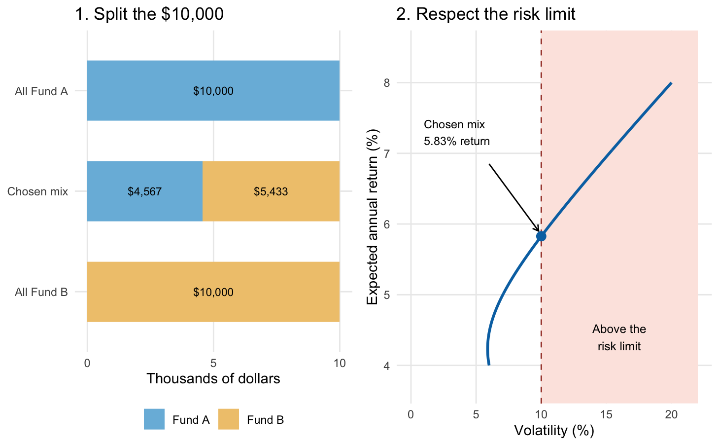
A stacked bar chart compares all Fund A, the chosen mix, and all Fund B. A risk-return curve highlights a chosen mix of 45.7 percent A and 54.3 percent B at 10 percent volatility and 5.83 percent expected return. Higher-volatility points lie in a shaded excluded region.
Figure 3.2: Left: three ways to split the same $10,000. Right: each point on the curve is a possible split. The selected mix has the highest expected return among points at or left of the 10% volatility limit. All inputs are illustrative.

Read the picture. Moving more money to Fund A moves us toward higher expected return, but eventually crosses the dashed risk limit. The chosen mix puts about $4,567 in A and $5,433 in B, for an expected return of 5.83% under these assumptions. All-A has a higher expected return, but is outside the allowed region.

Decision variable. Let \(w\) be the fraction of the $10,000 invested in Fund A. The remaining fraction, \(1-w\), is invested in Fund B.

Objective function. Maximize the expected annual return rate:

\[ \max_w\;R(w)=0.08w+0.04(1-w)=0.04+0.04w. \]

Constraints. All money is invested, with no borrowing or short selling, and portfolio volatility must not exceed 10%:

\[ 0\leq w\leq1,\qquad \sigma^2(w)\leq0.10^2=0.01. \]

The weights \(w\) and \(1-w\) already sum to one, so they enforce the $10,000 budget. Using the two standard deviations and the correlation of 0.10, the variance is explicitly

\[ \begin{aligned} \sigma^2(w) &=(0.20w)^2+[0.06(1-w)]^2\\ &\quad+2(0.10)(0.20)(0.06)w(1-w)\\ &=0.0412w^2-0.0048w+0.0036. \end{aligned} \]

Optimal solution. Expected return increases with \(w\), so choose the largest feasible weight. It lies on the risk boundary:

\[ 0.0412w^2-0.0048w+0.0036=0.01. \]

The positive root gives

\[ w^*\approx0.4566657,\qquad 1-w^*\approx0.5433343. \]

Invest approximately $4,566.66 in Fund A and $5,433.34 in Fund B. At the optimum,

\[ R(w^*)\approx0.0582666=5.82666\%,\qquad \sigma(w^*)=10\%. \]

Equivalently, this return corresponds to an expected annual gain of about $582.67 on the $10,000 investment. This is the unique global maximum: within \(0\leq w\leq1\), every feasible weight lies between zero and \(w^*\), and \(R(w)\) is strictly increasing.

Why an algorithm? In this two-fund example, uniroot() locates the boundary \(\sigma(w)=0.10\). With 20 funds, sector limits, and holding limits, many weights must be chosen together. Constrained portfolio solvers handle those interacting choices. Application context: MOSEK portfolio optimization cookbook.

Try explaining it: If the dashed risk limit moved to the right, would the best allowed mix contain more or less of Fund A?

The situation. A small factory has three orders, A, B, and C. Every order must go through Cutting, then Finishing. Each machine handles one order at a time. These illustrative processing times stay the same in both schedules:

Order Cutting Finishing
A 4 hours 1 hour
B 1 hour 4 hours
C 2 hours 2 hours

The computer’s job: choose the order of work so that all three orders finish as early as possible.

Code
factory_times <- data.frame(Job = c("A", "B", "C"),
                            Cutting = c(4, 1, 2), Finishing = c(1, 4, 2))
factory_schedule <- function(order, label) {
  cutting_free <- finishing_free <- 0
  tasks <- list()
  for (job in order) {
    duration <- factory_times[factory_times$Job == job, ]
    cut_start <- cutting_free
    cut_end <- cut_start + duration$Cutting
    finish_start <- max(cut_end, finishing_free)
    finish_end <- finish_start + duration$Finishing
    tasks[[job]] <- data.frame(
      Job = job, Machine = c("Cutting", "Finishing"),
      Start = c(cut_start, finish_start), End = c(cut_end, finish_end),
      Schedule = label
    )
    cutting_free <- cut_end
    finishing_free <- finish_end
  }
  do.call(rbind, tasks)
}
factory_tasks <- rbind(
  factory_schedule(c("A", "B", "C"), "1. Original: A-B-C | All done at hour 11"),
  factory_schedule(c("B", "C", "A"), "2. Improved: B-C-A | All done at hour 8")
)
factory_tasks$Machine <- factor(factory_tasks$Machine,
                                levels = c("Finishing", "Cutting"))
factory_ends <- aggregate(End ~ Schedule, factory_tasks, max)
ggplot(factory_tasks, aes(y = Machine, colour = Job)) +
  geom_segment(aes(x = Start, xend = End, yend = Machine),
               linewidth = 13, lineend = "butt") +
  geom_text(aes(x = (Start + End) / 2, label = Job),
            colour = "black", fontface = "bold", size = 4) +
  geom_vline(data = factory_ends, aes(xintercept = End),
             inherit.aes = FALSE, linetype = "dashed", colour = "grey40") +
  facet_wrap(~Schedule, ncol = 1) +
  scale_colour_manual(values = c(A = "#79BADD", B = "#F0C77C", C = "#A4D4B4")) +
  scale_x_continuous(breaks = 0:11, limits = c(0, 11.3)) +
  scale_y_discrete(expand = expansion(add = 0.7)) +
  labs(x = "Hours since work begins", y = NULL,
       title = "A Better Sequence Saves 3 Hours",
       subtitle = "Follow the same letter from Cutting to Finishing") +
  theme_minimal(base_size = 12) +
  theme(legend.position = "none", panel.grid.minor = element_blank(),
        panel.grid.major.y = element_blank())
Two Gantt charts compare A-B-C with B-C-A. In the original schedule, finishing starts at hour 4 and ends at hour 11. In the improved schedule, finishing starts at hour 1 and ends at hour 8. Each bar is labeled A, B, or C.
Figure 3.3: Same orders, same machines, same processing times. Changing the sequence reduces the last completion time from 11 to 8 hours. Empty horizontal space is idle time.

Read the picture. In the top schedule, Finishing waits four hours for A. In the bottom schedule, the short cutting step for B lets Finishing start after just one hour. The machines then overlap useful work more effectively. No machine runs faster; the sequence is better.

Decision variables. Choose a start time \(S_{jm}\) for each order \(j\in\{A,B,C\}\) on each machine \(m\in\{C,F\}\), where \(C\) means Cutting and \(F\) means Finishing. Also choose \(C_{\max}\), the time by which all orders must be complete. Let \(p_{jm}\) denote the fixed processing times in the table. All orders are available at time zero, and each operation runs without interruption once it starts.

Objective function. Minimize the last completion time (the makespan):

\[ \min_{\{S_{jm}\},\,C_{\max}}\;C_{\max}. \]

Constraints. The start times must satisfy four rules:

  1. Work cannot start before time zero: for every order \(j\) and machine \(m\),

    \[ S_{jm}\geq0. \]

  2. Cutting precedes Finishing: for each order \(j\),

    \[ S_{jF}\geq S_{jC}+p_{jC}. \]

  3. A machine cannot process two orders at once: for every pair of different orders \(j,k\) and each machine \(m\),

    \[ S_{jm}+p_{jm}\leq S_{km} \quad\text{or}\quad S_{km}+p_{km}\leq S_{jm}. \]

    In words, either \(j\) finishes before \(k\) starts, or \(k\) finishes before \(j\) starts. Choosing between these alternatives determines the job sequence.

  4. Every order finishes by \(C_{\max}\): for each order \(j\),

    \[ S_{jF}+p_{jF}\leq C_{\max}. \]

Optimal solution. One optimal sequence is B, then C, then A on both machines, with the following start and end times:

Order Cutting: start to end Finishing: start to end
B 0 to 1 1 to 5
C 1 to 3 5 to 7
A 3 to 7 7 to 8

All times are in hours. This feasible schedule achieves

\[ C_{\max}^*=8\text{ hours}. \]

Why is 8 hours globally optimal? Finishing requires \(1+4+2=7\) hours of work on a single machine. It cannot begin before hour 1, because even the shortest cutting operation takes 1 hour. Therefore every feasible schedule satisfies \(C_{\max}\geq1+7=8\). The schedule above reaches that lower bound, so no schedule can finish earlier. The original A-B-C schedule takes 11 hours.

For three orders, all six common orderings can also be checked. Larger factories require more systematic search; 20 jobs already give \(20!\approx2.43\times10^{18}\) possible orderings on one machine.

Why an algorithm? Constraint programming and mixed-integer optimization search subject to the rules. Simulated annealing and genetic algorithms can also explore valid schedules, though they do not certify the best possible result. This is a discrete choice problem: swapping two jobs is not a gradient step. Application context: OR-Tools job-shop scheduling.

Try explaining it: Find B in both panels. Why does doing its short cutting step early help the whole factory?

An online retailer has $100,000 for search advertising and social media. Start with a familiar decision: should it spend $50,000 on each, or split the money differently?

The situation. The first dollars spent on search work well, but that channel soon reaches many of the customers it can reach. Social media responds more gradually. We use two invented response curves to make the allocation problem visible; these are not measured campaign results.

Code
marketing_budget <- 100  # Thousands of dollars.
marketing_search <- function(spend) 900 * (1 - exp(-spend / 8))
marketing_social <- function(spend) 1600 * spend / (70 + spend)
marketing_orders <- function(search_spend) {
  marketing_search(search_spend) +
    marketing_social(marketing_budget - search_spend)
}
marketing_fit <- optimize(marketing_orders, c(0, marketing_budget),
                          maximum = TRUE)
marketing_comparison <- data.frame(
  Strategy = factor(c("Equal split", "Optimized"),
                    levels = c("Optimized", "Equal split")),
  Search = c(50, marketing_fit$maximum)
)
marketing_comparison$Social <- marketing_budget - marketing_comparison$Search
marketing_comparison$Orders <- marketing_orders(marketing_comparison$Search)

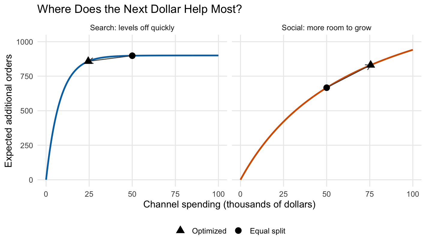
First, look at how each channel responds to spending. A steep curve means that another dollar produces a relatively large gain. A flat curve means that another dollar adds little.

Code
marketing_curves <- rbind(
  data.frame(Spend = seq(0, 100, length.out = 301),
             Channel = "Search: levels off quickly"),
  data.frame(Spend = seq(0, 100, length.out = 301),
             Channel = "Social: more room to grow")
)
marketing_curves$Orders <- ifelse(
  grepl("^Search", marketing_curves$Channel),
  marketing_search(marketing_curves$Spend),
  marketing_social(marketing_curves$Spend)
)
marketing_points <- rbind(
  data.frame(Spend = marketing_comparison$Search,
             Orders = marketing_search(marketing_comparison$Search),
             Strategy = marketing_comparison$Strategy,
             Channel = "Search: levels off quickly"),
  data.frame(Spend = marketing_comparison$Social,
             Orders = marketing_social(marketing_comparison$Social),
             Strategy = marketing_comparison$Strategy,
             Channel = "Social: more room to grow")
)
marketing_moves <- data.frame(
  Channel = c("Search: levels off quickly", "Social: more room to grow"),
  Spend = 50,
  Orders = c(marketing_search(50), marketing_social(50)),
  NewSpend = c(marketing_fit$maximum, 100 - marketing_fit$maximum),
  NewOrders = c(marketing_search(marketing_fit$maximum),
                marketing_social(100 - marketing_fit$maximum))
)
ggplot(marketing_curves, aes(Spend, Orders, colour = Channel)) +
  geom_line(linewidth = 1) +
  geom_segment(data = marketing_moves,
               aes(xend = NewSpend, yend = NewOrders),
               colour = "grey30", linewidth = 0.5,
               arrow = grid::arrow(length = grid::unit(0.1, "inches"))) +
  geom_point(data = marketing_points, aes(shape = Strategy),
             size = 3.5, colour = "black") +
  facet_wrap(~Channel, nrow = 1) +
  scale_colour_manual(values = c("#0072B2", "#D55E00")) +
  scale_shape_manual(values = c("Equal split" = 16, "Optimized" = 17)) +
  scale_y_continuous(limits = c(0, 1000)) +
  labs(x = "Channel spending (thousands of dollars)",
       y = "Expected additional orders", shape = NULL,
       title = "Where Does the Next Dollar Help Most?") +
  guides(colour = "none") +
  theme_minimal(base_size = 12) +
  theme(legend.position = "bottom", panel.grid.minor = element_blank())
Two response curves show diminishing returns. Search rises sharply and levels off, while social rises more gradually. An arrow moves search spending from 50 to 24.46 thousand dollars, and another moves social from 50 to 75.54 thousand dollars.
Figure 3.4: Illustrative response curves. Circles mark equal spending; triangles mark the optimized allocation. Arrows show the change: reduce search spending where the curve is flat and increase social spending where more gains remain.

Read the picture. At the equal split, search is already nearly flat. Moving some of that money to social loses relatively few search orders and gains more social orders. The optimizer keeps reallocating until the next dollar has the same marginal benefit in both channels.

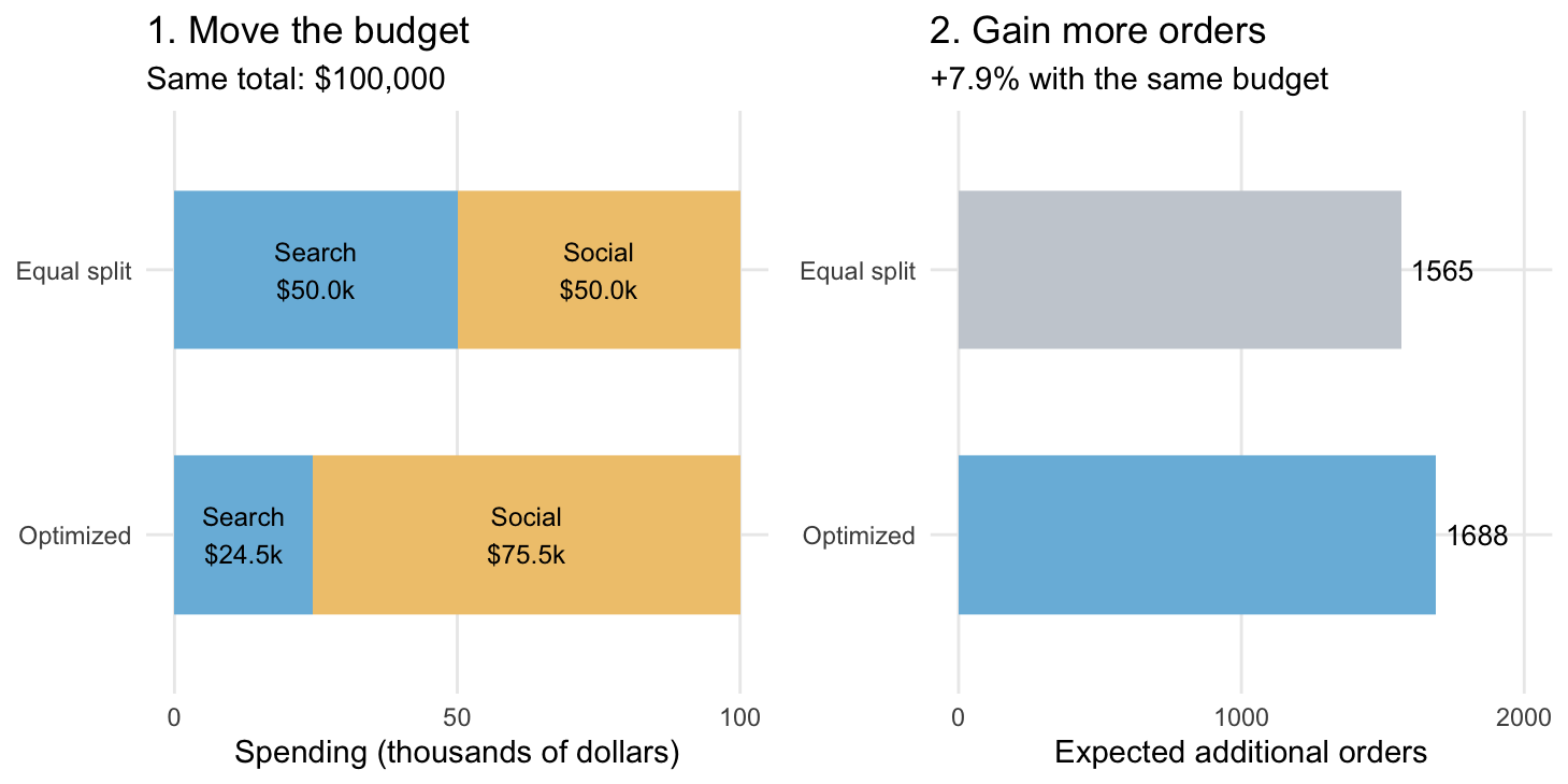
Now compare the decisions. The total budget stays at $100,000 in both rows. Only its allocation changes.

Code
marketing_spending <- rbind(
  data.frame(Strategy = marketing_comparison$Strategy, Channel = "Search",
             Spend = marketing_comparison$Search),
  data.frame(Strategy = marketing_comparison$Strategy, Channel = "Social",
             Spend = marketing_comparison$Social)
)
marketing_spending$Label <- sprintf("%s\n$%.1fk",
                                   marketing_spending$Channel,
                                   marketing_spending$Spend)
marketing_budget_plot <- ggplot(marketing_spending,
                                aes(Spend, Strategy, fill = Channel)) +
  geom_col(width = 0.6, position = position_stack(reverse = TRUE)) +
  geom_text(aes(label = Label), size = 3.2,
            position = position_stack(vjust = 0.5, reverse = TRUE)) +
  scale_fill_manual(values = c(Search = "#79BADD", Social = "#F0C77C")) +
  scale_x_continuous(limits = c(0, 100), breaks = c(0, 50, 100)) +
  labs(title = "1. Move the budget", subtitle = "Same total: $100,000",
       x = "Spending (thousands of dollars)",
       y = NULL) +
  theme_minimal(base_size = 11) +
  theme(legend.position = "none", panel.grid.minor = element_blank())
marketing_orders_plot <- ggplot(marketing_comparison,
                                aes(Orders, Strategy, fill = Strategy)) +
  geom_col(width = 0.6) +
  geom_text(aes(label = sprintf("%.0f", Orders)), hjust = -0.15, size = 3.5) +
  scale_fill_manual(values = c("Equal split" = "#C9CED5", "Optimized" = "#79BADD")) +
  scale_x_continuous(limits = c(0, 2000), breaks = c(0, 1000, 2000)) +
  labs(title = "2. Gain more orders", subtitle = "+7.9% with the same budget",
       x = "Expected additional orders", y = NULL) +
  theme_minimal(base_size = 11) +
  theme(legend.position = "none", panel.grid.minor = element_blank())
grid::grid.newpage()
grid::pushViewport(grid::viewport(layout = grid::grid.layout(1, 2)))
print(marketing_budget_plot,
      vp = grid::viewport(layout.pos.row = 1, layout.pos.col = 1))
print(marketing_orders_plot,
      vp = grid::viewport(layout.pos.row = 1, layout.pos.col = 2))
grid::popViewport()
Two equally long stacked budget bars compare 50-50 spending with 24.5-75.5 spending. Beside them, order bars increase from 1565 for the equal split to 1688 for the optimized allocation, a 7.9 percent increase.
Figure 3.5: A visual before-and-after comparison. The optimized split spends about $24,461 on search and $75,539 on social, producing about 123 more expected orders with the same budget under the illustrative model.

The change is from about 1,565 to 1,688 expected additional orders: approximately 123 extra orders, or 7.9%, without increasing spending.

Decision variables. Let \(s\) and \(u\) be spending on search and social advertising, respectively, in thousands of dollars. For example, \(s=25\) means $25,000 spent on search.

Objective function. Maximize the expected number of additional orders:

\[ \max_{s,u}\;F(s,u) =900(1-e^{-s/8})+1600\frac{u}{70+u}. \]

The first term is the search contribution and the second is the social contribution. We assume these contributions add without overlap and that all orders have the same value.

Constraints. Spend the full $100,000 budget, with neither channel receiving a negative amount:

\[ s\geq0,\qquad u\geq0,\qquad s+u=100. \]

There are no additional channel spending limits in this example. Substituting \(u=100-s\) gives the equivalent problem used by optimize():

\[ \max_{0\leq s\leq100}\;f(s) =900(1-e^{-s/8})+1600\frac{100-s}{170-s}. \]

Optimal solution. The best allocation is approximately

\[ s^*=24.46073,\qquad u^*=75.53927, \]

or $24,460.73 on search and $75,539.27 on social. Its objective value is

\[ F(s^*,u^*)\approx1688.1476\text{ expected additional orders}. \]

For comparison, equal spending gives \(F(50,50)\approx1564.9293\). The optimal allocation therefore adds about 123.2183 expected orders, a 7.87% increase with the same budget.

Why is this allocation optimal? Both response curves are strictly concave, so the feasible problem has a unique global maximum. The optimum lies inside \(0<s<100\) and solves

\[ f'(s)=112.5e^{-s/8}-\frac{112000}{(170-s)^2}=0. \]

At \(s^*\), both channels have the same marginal gain: approximately 5.2876 additional orders per $1,000 of spending. Shifting a small amount of money from one channel to the other can no longer improve the total.

Why an algorithm? Setting \(u=100-s\) leaves one adjustable number. optimize() searches for its best value. Here the total-response curve is strictly concave, so there is a unique maximum. With many channels and spending limits, this becomes a multivariate constrained problem.

Marketing tools such as Google’s Meridian apply this response-curve idea to budget allocation. In practice, the curves must be estimated and validated; the optimizer’s result depends on their accuracy. Application context: Meridian budget optimization.

Try explaining it: Point to the two equal-length budget bars. Where do the extra orders come from if no extra money is spent?
Examples are adapted from the following sources: