1  Matrix Representation and Notation

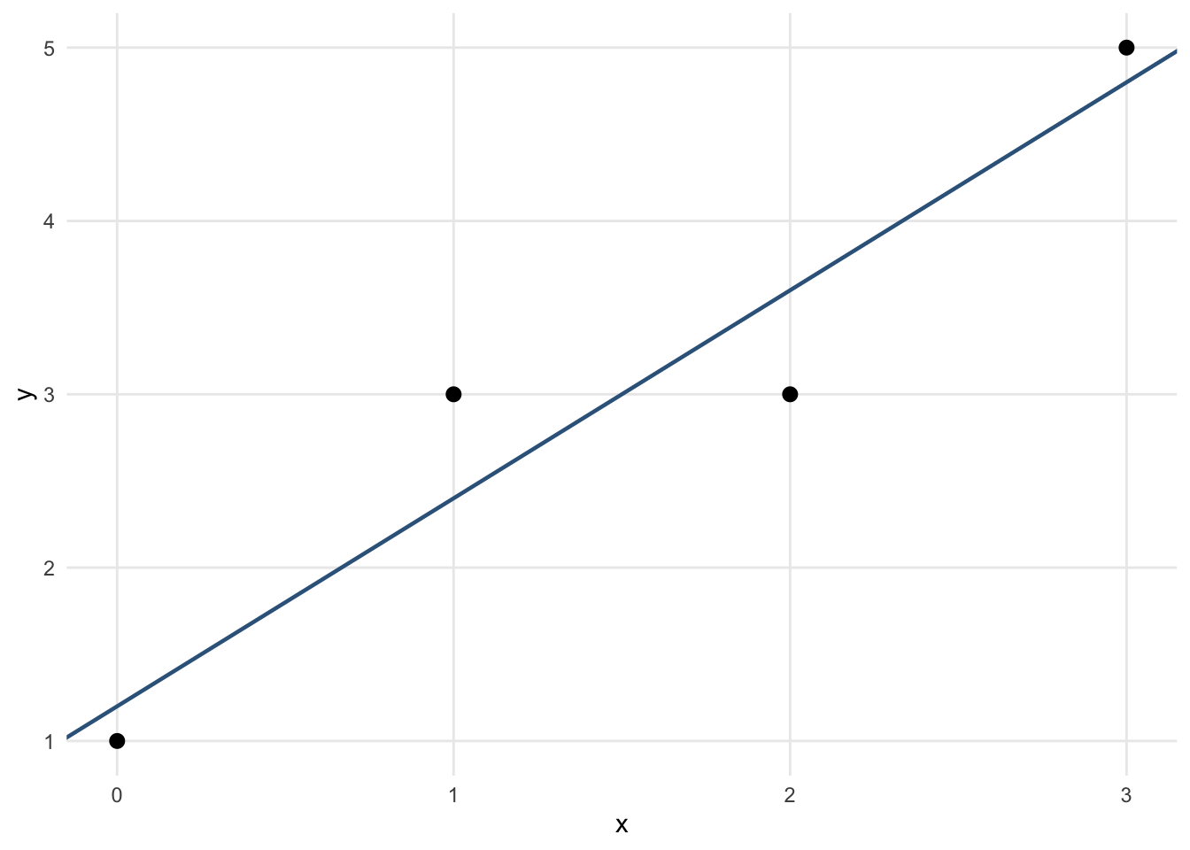
In this chapter, we introduce the mathematical language and statistical framework that will be used throughout the course. Our focus is on the notation of vectors and matrices, vectors of random variables, expectation and covariance operators, and the basic form of the linear regression model.

Learning Objectives

By the end of this chapter, students should be able to:

• use standard matrix notation for linear statistical models;
• distinguish between scalars, vectors, matrices, random variables, and random vectors;
• compute expectations and covariance matrices for random vectors;
• interpret the linear regression model in matrix form;
• understand why projection and least squares will play a central role in this course.

Reading

Recommended reading for this chapter:

• Seber and Lee (2003), Chapter 1:
  • 1.1 Notation
  • 1.2 Statistical Models
  • 1.3 Linear Regression Models
  • 1.4 Expectation and Covariance Operators
• Optional preview:
  • Chapter 2: Multivariate Normal Distribution

1.1 Why Linear Statistical Analysis?

Linear statistical analysis is one of the central foundations of graduate statistics. Many methods that at first look different are built on the same underlying structure:

• regression
• analysis of variance
• analysis of covariance
• prediction
• model comparison
• and parts of generalized linear modelling

A major goal of this course is to see these topics under a unified framework.

1.2 A unifying point of view

A large part of the course can be summarized by the model

\[ Y = X\beta + \varepsilon, \]

where

• \(Y\) is a response vector,
• \(X\) is a design matrix,
• \(\beta\) is an unknown parameter vector,
• \(\varepsilon\) is a random error vector.

This compact expression contains a great deal of statistical structure. Over the semester, we will study how to estimate \(\beta\), quantify uncertainty, test hypotheses, diagnose model failures, and make predictions.

1.3 Basic Notation

Scalars, vectors, and matrices

We use the following conventions throughout the course:

• scalars are written in lowercase italic letters, such as \(a\), \(b\), \(n\);
• vectors are written in bold lowercase letters, such as \(\mathbf{x}\), \(\mathbf{y}\);
• matrices are written in bold uppercase letters, such as \(\mathbf{X}\), \(\mathbf{A}\);
• random variables are often written in uppercase letters, such as \(Y\);
• realizations of random variables are written in lowercase letters, such as \(y\).

Univariate case

A random variable is univariate if it takes values in one dimension. We write

\[ X \in \mathbb{R}. \]

A realization, or observed value, of \(X\) is denoted by \(x\).

Some common quantities associated with a univariate random variable \(X\) include:

• Mean \[ \mu = \mathbb{E}(X). \]

• Variance \[ \sigma^2 = \operatorname{Var}(X) = \mathbb{E}\left[(X-\mu)^2\right]. \]

• \(k\)th moment \[ \mathbb{E}(X^k). \]

• Cumulative distribution function (CDF) \[ F(x) = P(X \leq x). \]

• Probability density function (PDF), for a continuous random variable, \[ f(x). \]

• Probability mass function (PMF), for a discrete random variable, \[ p(x) = P(X=x). \]

• Quantile \[ q_\alpha = F^{-1}(\alpha), \] where \(0<\alpha<1\).

For a random sample of size \(n\), we write

\[ X_1,X_2,\ldots,X_n, \]

with observed values

\[ x_1,x_2,\ldots,x_n. \]

The sample mean is

\[ \bar{x} = \frac{1}{n}\sum_{i=1}^n x_i, \]

and the sample variance is

\[ s^2 = \frac{1}{n-1} \sum_{i=1}^n (x_i-\bar{x})^2. \]

Multivariate case

A column vector in \(\mathbb{R}^n\) is written as

\[ \mathbf{x} = \begin{pmatrix} x_1 \\ x_2 \\ \vdots \\ x_n \end{pmatrix} = (x_1,x_2,\dots,x_n). \]

An \(n \times p\) matrix is written as

\[ \mathbf{X} = \begin{pmatrix} x_{11} & x_{12} & \cdots & x_{1p} \\ x_{21} & x_{22} & \cdots & x_{2p} \\ \vdots & \vdots & \ddots & \vdots \\ x_{n1} & x_{n2} & \cdots & x_{np} \end{pmatrix}. \]

Transpose, inverse, and rank

If \(\mathbf{A}\) is a matrix, then:

• \(\mathbf{A}^\top\) denotes its transpose;
• \(\mathbf{A}^{-1}\) denotes its inverse, when it exists;
• \(\mathrm{rank}(\mathbf{A})\) denotes its rank;
• \(\mathbf{I}_n\) denotes the \(n \times n\) identity matrix.

1.3.1 Inner product and norm

For vectors \(\mathbf{x}, \mathbf{y} \in \mathbb{R}^n\), the inner product is

\[ \mathbf{x}^\top \mathbf{y} = \sum_{i=1}^n x_i y_i. \]

For vectors \(\mathbf{x}, \mathbf{y} \in \mathbb{R}^n\), the inner product is

\[ \|\mathbf{x}\| = \sqrt{\mathbf{x}^\top \mathbf{x}}. \]

These ideas are fundamental because least squares estimation is based on minimizing squared Euclidean distance.

A random vector is a vector whose entries are random variables. For example,

\[ \mathbf{Y} = \begin{pmatrix} Y_1 \\ Y_2 \\ \vdots \\ Y_n \end{pmatrix} \]

is an \(n\)-dimensional random vector.

In linear models, the response is naturally treated as a random vector.

The mean vector of \(\mathbf{Y}\) is

\[ \mathbb{E}[\mathbf{Y}] = \begin{pmatrix} \mathbb{E}[Y_1] \\ \mathbb{E}[Y_2] \\ \vdots \\ \mathbb{E}[Y_n] \end{pmatrix}. \]

We often write \(\mathbb{E}[\mathbf{Y}] = \boldsymbol{\mu}.\)

The covariance matrix of \(\mathbf{Y}\) is

\[ \mathrm{Var}(\mathbf{Y}) = \mathbb{E}\left[ (\mathbf{Y} - \boldsymbol{\mu})(\mathbf{Y} - \boldsymbol{\mu})^\top \right]. \]

Equivalently,

\[ \mathrm{Var}(\mathbf{Y}) = \mathbb{E}[\mathbf{Y}\mathbf{Y}^\top] - \boldsymbol{\mu}\boldsymbol{\mu}^\top. \]

Suppose \(\mathbf{Y}=(Y_1, Y_2, Y_3)\).

Then the corresponding covariance matrix is

\[ \mathrm{Var}(\mathbf{Y}) = \begin{pmatrix} \mathrm{Var}(Y_1) & \mathrm{Cov}(Y_1,Y_2) & \mathrm{Cov}(Y_1,Y_3) \\ \mathrm{Cov}(Y_2,Y_1) & \mathrm{Var}(Y_2) & \mathrm{Cov}(Y_2,Y_3) \\ \mathrm{Cov}(Y_3,Y_1) & \mathrm{Cov}(Y_3,Y_2) & \mathrm{Var}(Y_3) \end{pmatrix}. \]

1.3.2 Expectation and Covariance Operators

If \(\mathbf{A}\) is a constant matrix and \(\mathbf{b}\) is a constant vector, then

\[ \mathbb{E}[\mathbf{A}\mathbf{Y} + \mathbf{b}] = \mathbf{A}\mathbb{E}[\mathbf{Y}] + \mathbf{b}. \]

This is one of the most useful identities in the course.

If \(\mathbf{A}\) is a constant matrix, then

\[ \mathrm{Var}(\mathbf{A}\mathbf{Y}) = \mathbf{A}\,\mathrm{Var}(\mathbf{Y})\,\mathbf{A}^\top. \]

More generally, if \(\mathbf{Y}\) and \(\mathbf{Z}\) are random vectors, then

\[ \mathrm{Cov}(\mathbf{A}\mathbf{Y}, \mathbf{B}\mathbf{Z}) = \mathbf{A}\,\mathrm{Cov}(\mathbf{Y},\mathbf{Z})\,\mathbf{B}^\top. \]

These formulas are essential for deriving the variance of estimators later.

If \(Y_1,\dots,Y_n\) are independent and each has variance \(\sigma^2\), then

\[ \mathrm{Var}(\mathbf{Y}) = \sigma^2 \mathbf{I}_n. \]

This is the most common starting assumption in classical linear regression.

1.4 Statistical Models

A statistical model is a set of probability distributions that may plausibly describe the data-generating mechanism.

1.4.1 General idea

Suppose we observe data \(y\) from a random quantity \(Y\). A model introduces assumptions about the distribution of \(Y\), often indexed by an unknown parameter \(\theta\).

For example:

\[ Y \sim N(\mu, \sigma^2) \]

with unknown parameters \(\mu\) and \(\sigma^2\).

In regression, the model is not only about the marginal distribution of the response but also about how the mean changes with explanatory variables.

1.4.2 Deterministic part and random part

A useful way to think about a statistical model is:

\[ \text{data} = \text{systematic part} + \text{random part}. \]

For linear regression, this becomes

\[ Y_i = \beta_0 + \beta_1 x_i + \varepsilon_i. \]

Here,

• \(\beta_0 + \beta_1 x_i\) is the systematic part;
• \(\varepsilon_i\) is the random part.

1.5 The Linear Regression Model

Perhaps the most simple model is the simple linear regression where there are only one independent variable and one response variable.

A simple linear regression model is defined as

\[ Y_i = \beta_0 + \beta_1 x_i + \varepsilon_i, \qquad i=1,\dots,n, \] with the typical assumption as

\[ \mathbb{E}[\varepsilon_i] = 0, \qquad \mathrm{Var}(\varepsilon_i) = \sigma^2, \qquad \mathrm{Cov}(\varepsilon_i,\varepsilon_j)=0 \text{ for } i \ne j. \]

Matrix form

We can write the model compactly as

\[ \mathbf{Y} = \mathbf{X}\boldsymbol{\beta} + \boldsymbol{\varepsilon}, \]

where

\[ \mathbf{Y} = \begin{pmatrix} Y_1 \\ Y_2 \\ \vdots \\ Y_n \end{pmatrix}, \qquad \mathbf{X} = \begin{pmatrix} 1 & x_1 \\ 1 & x_2 \\ \vdots & \vdots \\ 1 & x_n \end{pmatrix}, \qquad \boldsymbol{\beta} = \begin{pmatrix} \beta_0 \\ \beta_1 \end{pmatrix}, \qquad \boldsymbol{\varepsilon} = \begin{pmatrix} \varepsilon_1 \\ \varepsilon_2 \\ \vdots \\ \varepsilon_n \end{pmatrix}. \]

This notation will allow us to treat simple regression, multiple regression, ANOVA, and ANCOVA in one common language.

Under the same assumption,
\[ \mathbb{E}[\boldsymbol{\varepsilon}] = \mathbf{0} \qquad \text{and} \qquad \mathrm{Var}(\boldsymbol{\varepsilon}) = \sigma^2 \mathbf{I}_n, \] we have the following.

\[ \mathbb{E}[\mathbf{Y}] = \mathbf{X}\boldsymbol{\beta},\quad \mathrm{Var}(\mathbf{Y}) = \sigma^2 \mathbf{I}_n. \]

These are immediate consequences of the expectation and covariance rules above.

1.5.1 Geometry Preview

A central idea in linear regression is projection.

The fitted values \(\hat{\mathbf{Y}}\) will later be obtained by projecting \(\mathbf{Y}\) onto the column space of \(\mathbf{X}\).

The column space of \(\mathbf{X}\) is

\[ \mathcal{C}(\mathbf{X}) = \{ \mathbf{X}\boldsymbol{\beta} : \boldsymbol{\beta} \in \mathbb{R}^p \}. \] This is the set of all mean vectors that the model can represent.

1.6 Why projection matters

The least squares estimator chooses \(\hat{\boldsymbol{\beta}}\) so that

\[ \|\mathbf{Y} - \mathbf{X}\boldsymbol{\beta}\|^2 \]

is minimized.

So regression is not only algebra. It is also geometry.

Suppose we observe the following data:

\[ \begin{array}{c|cccc} x_i & 0 & 1 & 2 & 3 \\ \hline y_i & 1 & 3 & 3 & 5 \end{array} \]

Then

\[ \mathbf{Y} = \begin{pmatrix} 1 \\ 3 \\ 3 \\ 5 \end{pmatrix}, \qquad \mathbf{X} = \begin{pmatrix} 1 & 0 \\ 1 & 1 \\ 1 & 2 \\ 1 & 3 \end{pmatrix}. \]

We will learn next chapter that the least squares estimator is

\[ \hat{\boldsymbol{\beta}} = (\mathbf{X}^\top \mathbf{X})^{-1}\mathbf{X}^\top \mathbf{Y}. \]

For now, the main point is to understand how the model is written and how the data are represented in matrix form.

R code

x <- c(0, 1, 2, 3)
y <- c(1, 3, 3, 5)

mod <- lm(y ~ x)
summary(mod)

Call:
lm(formula = y ~ x)

Residuals:
   1    2    3    4 
-0.2  0.6 -0.6  0.2 

Coefficients:
            Estimate Std. Error t value Pr(>|t|)  
(Intercept)   1.2000     0.5292   2.268   0.1515  
x             1.2000     0.2828   4.243   0.0513 .
---
Signif. codes:  0 '***' 0.001 '**' 0.01 '*' 0.05 '.' 0.1 ' ' 1

Residual standard error: 0.6325 on 2 degrees of freedom
Multiple R-squared:    0.9, Adjusted R-squared:   0.85 
F-statistic:    18 on 1 and 2 DF,  p-value: 0.05132

# Inspecting the design matrix
model.matrix(mod)

  (Intercept) x
1           1 0
2           1 1
3           1 2
4           1 3
attr(,"assign")
[1] 0 1

# Fitted values and residuals
fitted(mod)

  1   2   3   4 
1.2 2.4 3.6 4.8 

residuals(mod)

   1    2    3    4 
-0.2  0.6 -0.6  0.2 

# quick plot
plot(x, y, pch = 19, xlab = "x", ylab = "y")
abline(mod, lwd = 2)

1.7 Discussion

1. Why is it helpful to write regression models in matrix form rather than only scalar notation?

2. What does the covariance matrix tell us that separate variances do not?

3. What is the interpretation of the column space of \(\mathbf{X}\)?

4. In what sense is regression a projection problem?

1.8 Practice Problems

Conceptual

1. Explain the difference between a random variable and a random vector.

2. Explain why \(\mathrm{Var}(\mathbf{Y})\) must be a symmetric matrix.

3. Give an example of a statistical model outside regression.

Computational

Let

\[ \mathbf{Y} = \begin{pmatrix} Y_1 \\ Y_2 \end{pmatrix} \]

with

\[ \mathbb{E}[\mathbf{Y}] = \begin{pmatrix} 1 \\ 2 \end{pmatrix}, \qquad \mathrm{Var}(\mathbf{Y}) = \begin{pmatrix} 4 & 1 \\ 1 & 9 \end{pmatrix}. \]

Let

\[ \mathbf{A} = \begin{pmatrix} 1 & 2 \\ 0 & 1 \end{pmatrix}, \qquad \mathbf{b} = \begin{pmatrix} 3 \\ -1 \end{pmatrix}. \]

Compute:

1. \(\mathbb{E}[\mathbf{A}\mathbf{Y} + \mathbf{b}]\)
2. \(\mathrm{Var}(\mathbf{A}\mathbf{Y})\)

Regression setup

For the model

\[ Y_i = \beta_0 + \beta_1 x_i + \varepsilon_i, \]

write out the matrices \(\mathbf{Y}\), \(\mathbf{X}\), \(\boldsymbol{\beta}\), and \(\boldsymbol{\varepsilon}\) for \(n=5\) observations.

1.9 Take home Practice

Complete the following:

• review matrix multiplication and transpose rules;
• derive \(\mathbb{E}[\mathbf{A}\mathbf{Y}+\mathbf{b}]\) from first principles;
• derive \(\mathrm{Var}(\mathbf{A}\mathbf{Y})\) using the definition of covariance;
• write the simple linear regression model in matrix form for a dataset of your choice;
• fit a simple regression in R and report:
• the estimated coefficients,
• fitted values,
• residuals,
• and a scatterplot with the fitted line.

1.10 Summary

This chapter introduced the notation and basic probabilistic tools needed for the rest of the course. We defined random vectors, mean vectors, covariance matrices, and the matrix form of the linear regression model. These ideas will support everything that follows.

Next chapter, we will study least squares estimation and the geometry of projection in more detail.

For some optional review of the matrix algebra, see Matrix Algebra Review.

Seber, George AF, and Alan J Lee. 2003. Linear Regression Analysis. John Wiley & Sons.