Introduction

This course develops a common language for statistical modelling: specify the research question, construct a design matrix, estimate a mean structure, quantify uncertainty, and check whether the assumptions are credible.

The core sequence covers matrix notation and least squares; normal distributions and quadratic forms; inference and model comparison; categorical predictors, contrasts, and experimental design; diagnostics, transformations, and weighting; and an introduction to generalized linear models for binary and count responses.

The final GLM unit keeps the same linear predictor while extending the response distribution and mean link. Logistic and Poisson regression provide practical examples. The Optional topic group contains supplementary material on rank-deficient models, automatic selection, correlated errors/GLS, GLM likelihood and computation, quantile regression, and mixed-effects models. Quantile regression and mixed-effects models are self-study readings for students who want to explore distributional features or grouped observations.

Lectures, homework, two in-class exams, and a final assessment develop both mathematical reasoning and reproducible analysis in R. Core tasks include interpreting estimates and intervals, identifying the experimental unit, and explaining the limits of an analysis.

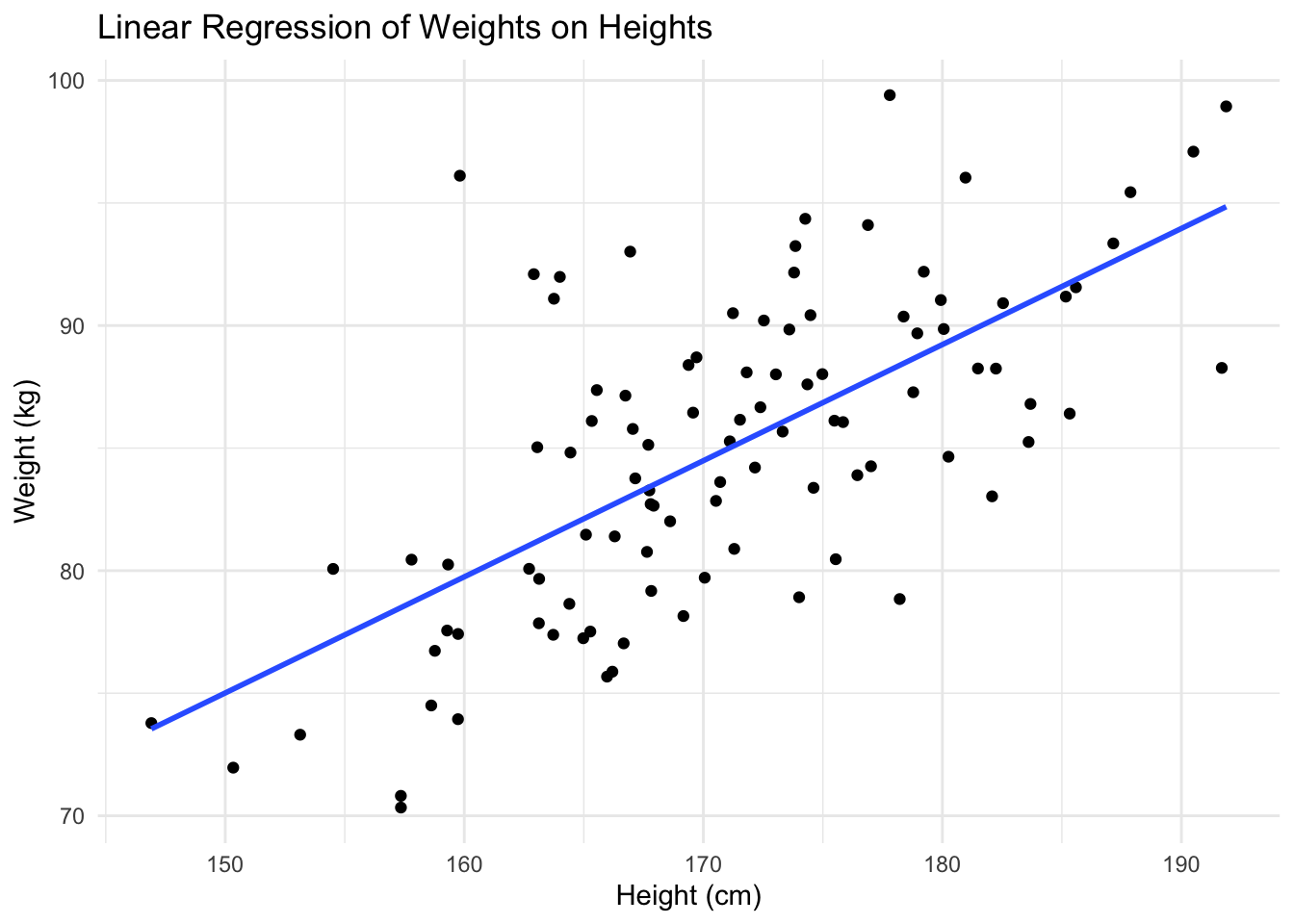
To illustrate the concepts we will be covering in this course, let’s consider a simple example. Suppose we have a data set of heights and weights of individuals. We want to understand the relationship between height and weight, and we can use linear regression to model this relationship.

# Load necessary libraries
library(ggplot2)
library(dplyr)

Attaching package: 'dplyr'

The following objects are masked from 'package:stats':

    filter, lag

The following objects are masked from 'package:base':

    intersect, setdiff, setequal, union

# Create a sample data set

set.seed(8561)

theme_set(theme_minimal(base_size = 11) +
            theme(legend.position = "bottom",
              panel.grid.minor = element_blank()))

n <- 100
heights <- rnorm(n, mean = 170, sd = 10)
weights <- 0.5 * heights + rnorm(n, mean = 0, sd = 5)
df <- data.frame(heights, weights)
head(df, 5)

   heights  weights
1 179.2812 88.01599
2 168.0474 76.10017
3 178.3029 83.46016
4 178.7006 82.01763
5 172.6678 92.84592

# Fit a linear regression model
model <- lm(weights ~ heights, data = df)
# Summarize the model
summary(model)

Call:
lm(formula = weights ~ heights, data = df)

Residuals:
     Min       1Q   Median       3Q      Max
-12.3303  -3.8998  -0.2191   3.2380  12.3478

Coefficients:
            Estimate Std. Error t value Pr(>|t|)
(Intercept) -1.92852    8.22226  -0.235    0.815
heights      0.50907    0.04857  10.481   <2e-16 ***
---
Signif. codes:  0 '***' 0.001 '**' 0.01 '*' 0.05 '.' 0.1 ' ' 1

Residual standard error: 5.251 on 98 degrees of freedom
Multiple R-squared:  0.5285,    Adjusted R-squared:  0.5237
F-statistic: 109.9 on 1 and 98 DF,  p-value: < 2.2e-16

# Plot the data and the fitted line
ggplot(df, aes(x = heights, y = weights)) +
  geom_point() +
  geom_smooth(method = "lm", formula = y ~ x, se = FALSE) +
  labs(title = "Linear Regression of Weights on Heights",
       x = "Height (cm)",
       y = "Weight (kg)")

In this example, we generated a data set of heights and weights, fitted a linear regression model to the data, and visualized the relationship between height and weight. This is just a simple example, but it illustrates the types of analyses we will be doing in this course. We will be covering much more complex models and data sets as we progress through the semester.

Throughout the course, we will be using R programming software.