In this chapter, we study one of the fundamental ideas in linear models: least squares estimation .
Recall that the linear model is
\[
\mathbf{Y}
=
\mathbf{X}\boldsymbol{\beta}
+
\boldsymbol{\varepsilon}.
\]
The unknown parameter vector \(\boldsymbol{\beta}\) determines the mean structure of the response. Given observed data, our first goal is to estimate \(\boldsymbol{\beta}\) .
The central idea of least squares is simple:
Choose the value of \(\boldsymbol{\beta}\) for which the fitted response \(\mathbf{X}\boldsymbol{\beta}\) is as close as possible to the observed response \(\mathbf{Y}\) .
This optimization problem leads to the normal equations , the least squares estimator , and a useful geometric interpretation in terms of orthogonal projection .
Learning Objectives
By the end of this chapter, students should be able to:
formulate least squares estimation as an optimization problem;
define the residual sum of squares;
derive the normal equations;
obtain the least squares estimator when \(\mathbf{X}\) has full column rank;
explain the role of the column space \(\mathcal{C}(\mathbf{X})\) ;
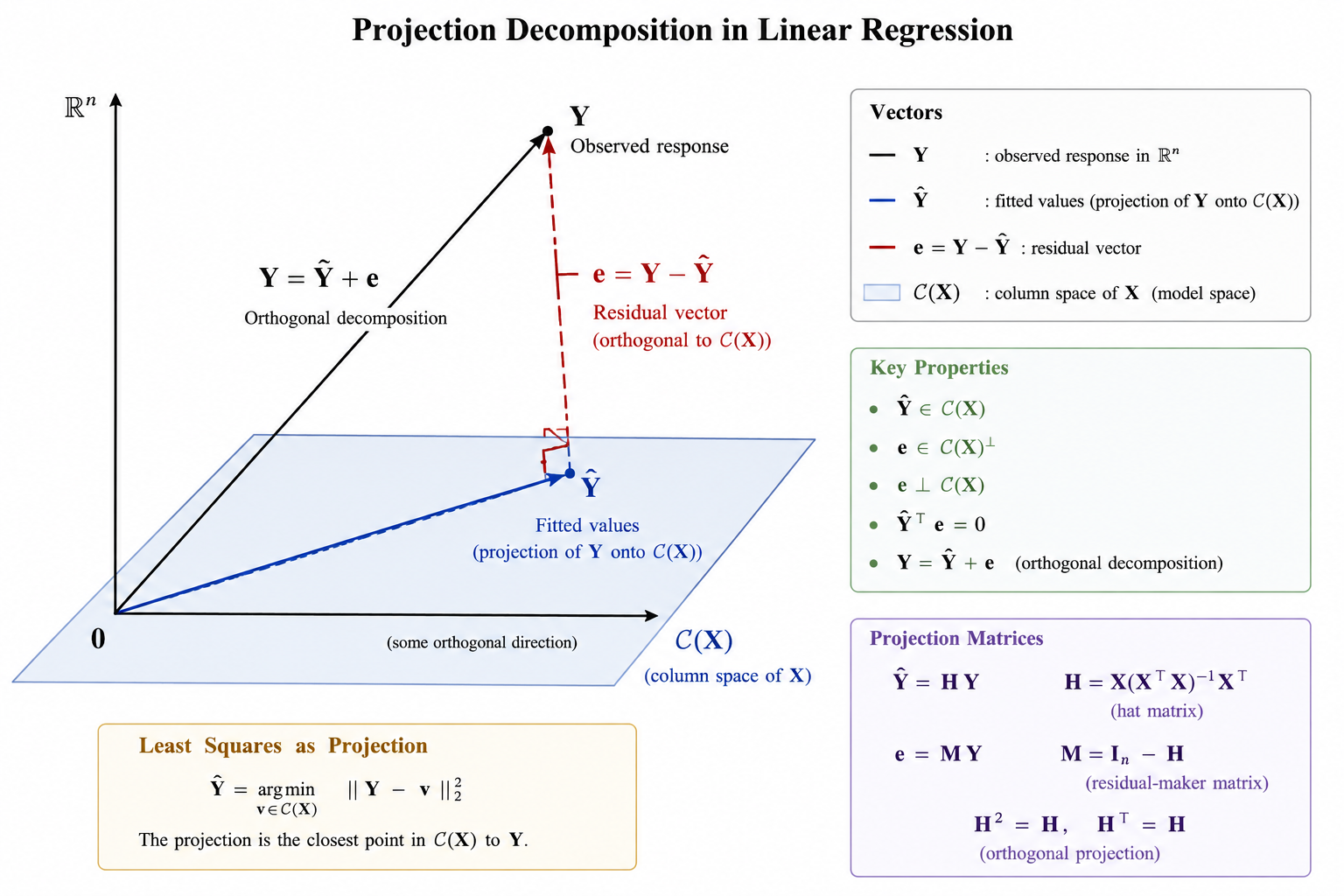
interpret fitted values as an orthogonal projection;
explain why residuals are orthogonal to the model space;
define and interpret the hat matrix and residual-maker matrix;
verify symmetry and idempotence of projection matrices;
explain the decomposition \(\mathbf{Y}=\hat{\mathbf{Y}}+\mathbf{e}\) ;
distinguish the uniqueness of \(\hat{\boldsymbol{\beta}}\) from the uniqueness of the fitted values.
Reading
Recommended reading for this week:
Seber and Lee:
Chapter 3: sections on least squares estimation
Montgomery, Peck, and Vining:
introductory sections on estimation in linear regression
Recall from Week 1 , the linear model can be written as
\[
\mathbf{Y}
=
\mathbf{X}\boldsymbol{\beta}
+
\boldsymbol{\varepsilon},
\]
where
\(\mathbf{Y}\) is an \(n\times 1\) response vector;\(\mathbf{X}\) is an \(n\times p\) design matrix;\(\boldsymbol{\beta}\) is a \(p\times 1\) parameter vector;\(\boldsymbol{\varepsilon}\) is an \(n\times 1\) error vector.
The design matrix may be written as
\[
\mathbf{X}
=
\begin{pmatrix}
\mathbf{x}_1^\top\\
\mathbf{x}_2^\top\\
\vdots\\
\mathbf{x}_n^\top
\end{pmatrix},
\]
where \(\mathbf{x}_i\in\mathbb{R}^p\) contains the predictors associated with observation \(i\) .
Thus,
\[
Y_i
=
\mathbf{x}_i^\top\boldsymbol{\beta}
+
\varepsilon_i,
\qquad
i=1,\ldots,n.
\]
Under the classical linear model, we often assume
\[
\mathbb{E}(\boldsymbol{\varepsilon})
=
\mathbf{0},
\qquad
\operatorname{Var}(\boldsymbol{\varepsilon})
=
\sigma^2\mathbf{I}_n.
\]
Consequently,
\[
\mathbb{E}(\mathbf{Y})
=
\mathbf{X}\boldsymbol{\beta},
\qquad
\operatorname{Var}(\mathbf{Y})
=
\sigma^2\mathbf{I}_n.
\]
The least squares estimator is defined through the optimization problem
\[
\min_{\boldsymbol{\beta}}
\left\|
\mathbf{Y}-\mathbf{X}\boldsymbol{\beta}
\right\|_2^2.
\]
No distributional assumption on \(\boldsymbol{\varepsilon}\) is required to define or compute the least squares estimator.
Assumptions such as
\[
\mathbb{E}(\boldsymbol{\varepsilon})=\mathbf{0}
\]
and
\[
\operatorname{Var}(\boldsymbol{\varepsilon})
=
\sigma^2\mathbf{I}_n
\]
are needed when we study the statistical properties of the estimator.
Normality will be introduced later when we study exact finite-sample inference.
The Least Squares Criterion
Motivation
For any candidate value \(\boldsymbol{\beta}\) , the corresponding fitted vector is
\[
\mathbf{X}\boldsymbol{\beta}.
\]
The discrepancy between the observed response \(\mathbf{Y}\) and this candidate fit is
\[
\mathbf{Y}-\mathbf{X}\boldsymbol{\beta}.
\]
A natural idea is to choose \(\boldsymbol{\beta}\) so that this discrepancy is as small as possible.
To measure its size, we use the squared Euclidean norm.
Residual Sum of Squares
The residual sum of squares associated with a candidate \(\boldsymbol{\beta}\) is
\[
S(\boldsymbol{\beta})
=
\left\|
\mathbf{Y}-\mathbf{X}\boldsymbol{\beta}
\right\|_2^2.
\]
Equivalently,
\[
S(\boldsymbol{\beta})
=
(\mathbf{Y}-\mathbf{X}\boldsymbol{\beta})^\top
(\mathbf{Y}-\mathbf{X}\boldsymbol{\beta}).
\]
In scalar notation,
\[
S(\boldsymbol{\beta})
=
\sum_{i=1}^n
\left(
Y_i-\mathbf{x}_i^\top\boldsymbol{\beta}
\right)^2.
\]
This last expression explains the name least squares : we choose \(\boldsymbol{\beta}\) to make the sum of the squared discrepancies as small as possible.
We therefore define
\[
\hat{\boldsymbol{\beta}}
=
\arg\min_{\boldsymbol{\beta}\in\mathbb{R}^p}
S(\boldsymbol{\beta}).
\]
Definition 2.1 (Least Squares Estimator) least squares estimator is any value \(\hat{\boldsymbol{\beta}}\) satisfying
\[
S(\hat{\boldsymbol{\beta}})
\leq
S(\boldsymbol{\beta})
\]
for every \(\boldsymbol{\beta}\in\mathbb{R}^p\) .
Example 2.1 (LSE for Simple Linear Regression)
\[
Y_i = \beta_0 + \beta_1 x_i + \varepsilon_i,
\qquad i=1,\ldots,n,
\]
where
\[
\mathbb{E}[\varepsilon_i]=0,
\qquad
\operatorname{Var}(\varepsilon_i)=\sigma^2.
\]
The fitted value at \(x_i\) is
\[
\hat{Y}_i
=
\beta_0+\beta_1 x_i.
\]
The corresponding residual is
\[
e_i
=
Y_i-\beta_0-\beta_1x_i.
\]
The least squares method chooses \(\beta_0\) and \(\beta_1\) to minimize the sum of squared residuals
\[
S(\beta_0,\beta_1)
=
\sum_{i=1}^n
\left(
Y_i-\beta_0-\beta_1x_i
\right)^2.
\]
Derivation of the Normal Equations
To minimize \(S(\beta_0,\beta_1)\) , differentiate with respect to \(\beta_0\) and \(\beta_1\) .
For \(\beta_0\) ,
\[
\frac{\partial S}{\partial\beta_0}
=
-2
\sum_{i=1}^n
\left(
Y_i-\beta_0-\beta_1x_i
\right).
\]
Setting this equal to zero gives
\[
\sum_{i=1}^n
\left(
Y_i-\hat{\beta}_0-\hat{\beta}_1x_i
\right)
=
0.
\]
Therefore,
\[
\sum_{i=1}^nY_i
=
n\hat{\beta}_0
+
\hat{\beta}_1\sum_{i=1}^nx_i.
\]
Dividing by \(n\) ,
\[
\bar{Y}
=
\hat{\beta}_0
+
\hat{\beta}_1\bar{x},
\]
so
\[
\boxed{
\hat{\beta}_0
=
\bar{Y}
-
\hat{\beta}_1\bar{x}
}.
\]
For \(\beta_1\) ,
\[
\frac{\partial S}{\partial\beta_1}
=
-2
\sum_{i=1}^n
x_i
\left(
Y_i-\beta_0-\beta_1x_i
\right).
\]
Setting this equal to zero gives
\[
\sum_{i=1}^n
x_i
\left(
Y_i-\hat{\beta}_0-\hat{\beta}_1x_i
\right)
=
0.
\]
Hence,
\[
\sum_{i=1}^n x_iY_i
=
\hat{\beta}_0\sum_{i=1}^nx_i
+
\hat{\beta}_1\sum_{i=1}^nx_i^2.
\]
Substituting
\[
\hat{\beta}_0
=
\bar{Y}-\hat{\beta}_1\bar{x},
\]
we obtain
\[
\sum_{i=1}^n x_iY_i
=
\left(
\bar{Y}-\hat{\beta}_1\bar{x}
\right)
\sum_{i=1}^nx_i
+
\hat{\beta}_1\sum_{i=1}^nx_i^2.
\]
Since
\[
\sum_{i=1}^n x_i
=
n\bar{x},
\]
we have
\[
\sum_{i=1}^n x_iY_i
-
n\bar{x}\bar{Y}
=
\hat{\beta}_1
\left(
\sum_{i=1}^nx_i^2
-
n\bar{x}^2
\right).
\]
Using
\[
\sum_{i=1}^n
(x_i-\bar{x})(Y_i-\bar{Y})
=
\sum_{i=1}^nx_iY_i
-
n\bar{x}\bar{Y},
\]
and
\[
\sum_{i=1}^n
(x_i-\bar{x})^2
=
\sum_{i=1}^nx_i^2
-
n\bar{x}^2,
\]
we obtain
\[
\boxed{
\hat{\beta}_1
=
\frac{
\sum_{i=1}^n
(x_i-\bar{x})(Y_i-\bar{Y})
}{
\sum_{i=1}^n
(x_i-\bar{x})^2
}
}.
\]
Therefore,
\[
\boxed{
\hat{\beta}_0
=
\bar{Y}
-
\hat{\beta}_1\bar{x}
}.
\]
Alternative Notation
It is common to define
\[
S_{xx}
=
\sum_{i=1}^n
(x_i-\bar{x})^2
\]
and
\[
S_{xy}
=
\sum_{i=1}^n
(x_i-\bar{x})(Y_i-\bar{Y}).
\]
Then
\[
\boxed{
\hat{\beta}_1
=
\frac{S_{xy}}{S_{xx}}
}
\]
and
\[
\boxed{
\hat{\beta}_0
=
\bar{Y}
-
\frac{S_{xy}}{S_{xx}}\bar{x}
}.
\]
Thus, the fitted regression line is
\[
\boxed{
\hat{Y}_i
=
\hat{\beta}_0
+
\hat{\beta}_1x_i
}.
\]
Derivation of the Least Squares Estimator in a matrix form
Expansion of the Criterion Starting from
\[
S(\boldsymbol{\beta})
=
(\mathbf{Y}-\mathbf{X}\boldsymbol{\beta})^\top
(\mathbf{Y}-\mathbf{X}\boldsymbol{\beta}),
\]
we expand:
\[\begin{align*}
S(\boldsymbol{\beta})
&=
\mathbf{Y}^\top\mathbf{Y}
-
\mathbf{Y}^\top\mathbf{X}\boldsymbol{\beta}
-
\boldsymbol{\beta}^\top\mathbf{X}^\top\mathbf{Y}
+
\boldsymbol{\beta}^\top
\mathbf{X}^\top\mathbf{X}
\boldsymbol{\beta}.
\end{align*}\]
Because
\[
\mathbf{Y}^\top\mathbf{X}\boldsymbol{\beta}
\]
is a scalar,
\[
\mathbf{Y}^\top\mathbf{X}\boldsymbol{\beta}
=
\boldsymbol{\beta}^\top\mathbf{X}^\top\mathbf{Y}.
\]
Therefore,
\[
\boxed{
S(\boldsymbol{\beta})
=
\mathbf{Y}^\top\mathbf{Y}
-
2\boldsymbol{\beta}^\top
\mathbf{X}^\top\mathbf{Y}
+
\boldsymbol{\beta}^\top
\mathbf{X}^\top\mathbf{X}
\boldsymbol{\beta}.
}
\]
Derivation of the Normal Equations
Differentiate \(S(\boldsymbol{\beta})\) with respect to \(\boldsymbol{\beta}\) :
\[
\frac{\partial S(\boldsymbol{\beta})}
{\partial\boldsymbol{\beta}}
=
-2\mathbf{X}^\top\mathbf{Y}
+
2\mathbf{X}^\top\mathbf{X}\boldsymbol{\beta}.
\]
At a minimum, the gradient is zero, so
\[
-2\mathbf{X}^\top\mathbf{Y}
+
2\mathbf{X}^\top
\mathbf{X}\hat{\boldsymbol{\beta}}
=
\mathbf{0}.
\]
Thus,
\[
\boxed{
\mathbf{X}^\top\mathbf{X}
\hat{\boldsymbol{\beta}}
=
\mathbf{X}^\top\mathbf{Y}.
}
\]
These are called the normal equations .
The normal equations can be written as
\[
\mathbf{X}^\top
\left(
\mathbf{Y}
-
\mathbf{X}\hat{\boldsymbol{\beta}}
\right)
=
\mathbf{0}.
\]
Later we will define
\[
\mathbf{e}
=
\mathbf{Y}
-
\mathbf{X}\hat{\boldsymbol{\beta}}.
\]
Therefore,
\[
\mathbf{X}^\top\mathbf{e}
=
\mathbf{0}.
\]
This means that \(\mathbf{e}\) is perpendicular, or normal , to the column space of \(\mathbf{X}\) .
Thus, the word normal is being used in its geometric sense.
Why is the Stationary Point a Minimum?
The Hessian of the least squares criterion is
\[
\nabla^2 S(\boldsymbol{\beta})
=
2\mathbf{X}^\top\mathbf{X}.
\]
For any \(\mathbf{a}\in\mathbb{R}^p\) ,
\[
\mathbf{a}^\top
\mathbf{X}^\top\mathbf{X}
\mathbf{a}
=
(\mathbf{X}\mathbf{a})^\top
(\mathbf{X}\mathbf{a})
=
\|\mathbf{X}\mathbf{a}\|_2^2
\geq 0.
\]
Therefore, \(\mathbf{X}^\top\mathbf{X}\) is positive semidefinite, and \(S(\boldsymbol{\beta})\) is a convex function.
If \(\mathbf{X}\) has full column rank, then for every \(\mathbf{a}\neq\mathbf{0}\) ,
\[
\mathbf{X}\mathbf{a}\neq\mathbf{0},
\]
and hence
\[
\mathbf{a}^\top
\mathbf{X}^\top\mathbf{X}
\mathbf{a}
>
0.
\]
Thus, \(\mathbf{X}^\top\mathbf{X}\) is positive definite and the least squares minimizer is unique.
A vector \(\hat{\boldsymbol{\beta}}\) minimizes
\[
S(\boldsymbol{\beta})
=
\left\|
\mathbf{Y}
-
\mathbf{X}\boldsymbol{\beta}
\right\|_2^2
\]
if and only if it satisfies the normal equations
\[
\mathbf{X}^\top\mathbf{X}
\hat{\boldsymbol{\beta}}
=
\mathbf{X}^\top\mathbf{Y}.
\]
If \(\mathbf{X}\) has full column rank,
\[
\operatorname{rank}(\mathbf{X})=p,
\]
then \(\mathbf{X}^\top\mathbf{X}\) is invertible and the least squares estimator is unique:
\[
\boxed{
\hat{\boldsymbol{\beta}}
=
(\mathbf{X}^\top\mathbf{X})^{-1}
\mathbf{X}^\top\mathbf{Y}.
}
\]
This is commonly called the ordinary least squares estimator , or OLS estimator .
The expression
\[
(\mathbf{X}^\top\mathbf{X})^{-1}
\]
exists if and only if \(\mathbf{X}\) has full column rank:
\[
\operatorname{rank}(\mathbf{X})=p.
\]
This means that the columns of \(\mathbf{X}\) are linearly independent.
If they are linearly dependent, then \(\mathbf{X}^\top\mathbf{X}\) is singular and the inverse does not exist.
We will return to this issue later.
Example 2.2 (LSE for Simple Linear Regression continue) Example 2.1 , we know the expression of the LSE \(\hat{\boldsymbol{\beta}}\) . Here, we want to see its connection to the matrix Form.
For simple linear regression,
\[
\mathbf{Y}
=
\begin{pmatrix}
Y_1\\
Y_2\\
\vdots\\
Y_n
\end{pmatrix},
\qquad
\mathbf{X}
=
\begin{pmatrix}
1 & x_1\\
1 & x_2\\
\vdots & \vdots\\
1 & x_n
\end{pmatrix},
\qquad
\boldsymbol{\beta}
=
\begin{pmatrix}
\beta_0\\
\beta_1
\end{pmatrix}.
\]
The general least squares estimator is
\[
\hat{\boldsymbol{\beta}}
=
(\mathbf{X}^\top\mathbf{X})^{-1}
\mathbf{X}^\top\mathbf{Y}.
\]
For simple linear regression,
\[
\mathbf{X}^\top\mathbf{X}
=
\begin{pmatrix}
n & \sum_{i=1}^n x_i\\
\sum_{i=1}^n x_i & \sum_{i=1}^n x_i^2
\end{pmatrix},
\]
and
\[
\mathbf{X}^\top\mathbf{Y}
=
\begin{pmatrix}
\sum_{i=1}^nY_i\\
\sum_{i=1}^nx_iY_i
\end{pmatrix}.
\]
Therefore,
\[
\hat{\boldsymbol{\beta}}
=
\begin{pmatrix}
\hat{\beta}_0\\
\hat{\beta}_1
\end{pmatrix}
=
(\mathbf{X}^\top\mathbf{X})^{-1}
\mathbf{X}^\top\mathbf{Y},
\]
which gives exactly
\[
\boxed{
\hat{\beta}_1
=
\frac{
\sum_{i=1}^n(x_i-\bar{x})(Y_i-\bar{Y})
}{
\sum_{i=1}^n(x_i-\bar{x})^2
}
}
\]
and
\[
\boxed{
\hat{\beta}_0
=
\bar{Y}-\hat{\beta}_1\bar{x}
}.
\]
Hence,
The familiar simple linear regression formulas for \(\hat{\beta}_0\) and \(\hat{\beta}_1\) are special cases of the general matrix LSE
\[
\hat{\boldsymbol{\beta}}
=
(\mathbf{X}^\top\mathbf{X})^{-1}
\mathbf{X}^\top\mathbf{Y}.
\]
Geometric Interpretation of Least Squares
The algebraic derivation gives us the estimator. However, the geometry explains why least squares has its important properties.
The column space of \(\mathbf{X}\) is
\[
\mathcal{C}(\mathbf{X})
=
\left\{
\mathbf{X}\boldsymbol{\beta}
:
\boldsymbol{\beta}\in\mathbb{R}^p
\right\}.
\]
Thus, \(\mathcal{C}(\mathbf{X})\) is the set of all response vectors that can be represented exactly by the linear model.
If \(\mathbf{X}\) has full column rank \(p\) , then
\[
\dim\left\{\mathcal{C}(\mathbf{X})\right\}=p.
\]
Because \(\mathbf{X}\) has \(n\) rows,
\[
\mathcal{C}(\mathbf{X})
\subseteq
\mathbb{R}^n.
\]
Least Squares as Projection
The fitted value vector is
\[
\hat{\mathbf{Y}}
=
\mathbf{X}\hat{\boldsymbol{\beta}}.
\]
Because
\[
\hat{\mathbf{Y}}
\in
\mathcal{C}(\mathbf{X}),
\]
least squares chooses the vector in \(\mathcal{C}(\mathbf{X})\) that is closest to the observed vector \(\mathbf{Y}\) .
That is,
\[
\hat{\mathbf{Y}}
=
\arg\min_{\mathbf{v}\in\mathcal{C}(\mathbf{X})}
\|\mathbf{Y}-\mathbf{v}\|_2^2.
\]
Therefore, \(\hat{\mathbf{Y}}\) is the orthogonal projection of \(\mathbf{Y}\) onto \(\mathcal{C}(\mathbf{X})\) .
So we can say that the fitted vector \(\hat{\mathbf{Y}}\) is constrained to live in the model space generated by the predictors. Least squares finds the point in that space closest to the observed data vector \(\mathbf{Y}\) .
Definition 2.2 (Orthogonality) \(\mathbf{u},\mathbf{v}\in\mathbb{R}^n\) are said to be orthogonal if their inner product is zero:
\[
\mathbf{u}^\top\mathbf{v}=0.
\]
We write
\[
\mathbf{u}\perp\mathbf{v}.
\]
Geometrically, two nonzero vectors are orthogonal if the angle between them is \(90^\circ\) .
Definition 2.3 (Residual Vector) residual vector
\[
\boxed{
\mathbf{e}
=
\mathbf{Y}
-
\hat{\mathbf{Y}}
=
\mathbf{Y}
-
\mathbf{X}\hat{\boldsymbol{\beta}}.
}
\]
The individual residuals are
\[
e_i
=
Y_i-\hat{Y}_i,
\qquad
i=1,\ldots,n.
\]
Geometrically, \(\mathbf{e}\) is the component of \(\mathbf{Y}\) that is orthogonal to the model space \(\mathcal{C}(\mathbf{X})\) .
Proposition 2.1 (Orthogonality of the Residuals) \(\mathbf{X}^\top\mathbf{X}\hat{\boldsymbol{\beta}}
=
\mathbf{X}^\top\mathbf{Y}.\) If we rearrange, we have \(\mathbf{X}^\top\left(\mathbf{Y}-\mathbf{X}\hat{\boldsymbol{\beta}}\right)=\mathbf{0}.\)
Since the residual vector is
\[
\mathbf{e}
=
\mathbf{Y}
-
\hat{\mathbf{Y}}
=
\mathbf{Y}
-
\mathbf{X}\hat{\boldsymbol{\beta}},
\]
we obtain the fundamental least squares property
\[
\boxed{
\mathbf{X}^\top\mathbf{e}
=
\mathbf{0}.
}
\]
To understand what this means, write the design matrix as
\[
\mathbf{X}
=
\begin{pmatrix}
\mathbf{x}^{(1)}
&
\mathbf{x}^{(2)}
&
\cdots
&
\mathbf{x}^{(p)}
\end{pmatrix},
\]
where \(\mathbf{x}^{(j)}\) is the \(j\) th column of \(\mathbf{X}\) .
Then
\[
\mathbf{X}^\top\mathbf{e}
=
\begin{pmatrix}
(\mathbf{x}^{(1)})^\top\mathbf{e}\\
(\mathbf{x}^{(2)})^\top\mathbf{e}\\
\vdots\\
(\mathbf{x}^{(p)})^\top\mathbf{e}
\end{pmatrix}
=
\mathbf{0}.
\]
Therefore,
\[
(\mathbf{x}^{(j)})^\top\mathbf{e}
=
0,
\qquad
j=1,\ldots,p.
\]
Thus, the residual vector is orthogonal to every column of \(\mathbf{X}\) .
Because the column space \(\mathcal{C}(\mathbf{X})\) consists of all linear combinations of the columns of \(\mathbf{X}\) , it follows that
\[
\boxed{
\mathbf{e}
\perp
\mathcal{C}(\mathbf{X}).
}
\]
Intuition. The columns of \(\mathbf{X}\) represent all directions that the linear model is allowed to use. After least squares has chosen the best fitted value, the remaining error \(\mathbf{e}\) has no component left in any of these directions. Otherwise, we could move the fitted value within \(\mathcal{C}(\mathbf{X})\) and reduce the residual sum of squares further.
Proposition 2.2 (Fundamental Orthogonal Decomposition)
\[
\hat{\mathbf{Y}}
=
\mathbf{X}\hat{\boldsymbol{\beta}}.
\]
Therefore,
\[
\boxed{
\hat{\mathbf{Y}}
\in
\mathcal{C}(\mathbf{X}).
}
\]
In other words, \(\hat{\mathbf{Y}}\) must lie in the space generated by the columns of \(\mathbf{X}\) .
Since
\[
\mathbf{e}
=
\mathbf{Y}
-
\hat{\mathbf{Y}},
\]
we can write
\[
\boxed{
\mathbf{Y}
=
\hat{\mathbf{Y}}
+
\mathbf{e}.
}
\]
The two components satisfy
\[
\hat{\mathbf{Y}}
\in
\mathcal{C}(\mathbf{X})
\]
and
\[
\mathbf{e}
\in
\mathcal{C}(\mathbf{X})^\perp.
\]
Hence,
\[
\boxed{
\hat{\mathbf{Y}}^\top\mathbf{e}
=
0.
}
\]
Geometrically, least squares projects \(\mathbf{Y}\) onto the column space of \(\mathbf{X}\) :
\[
\mathbf{Y}
=
\underbrace{\hat{\mathbf{Y}}}_{\text{part explained by the model}}
+
\underbrace{\mathbf{e}}_{\text{part orthogonal to the model space}}.
\]
Because the two components are orthogonal, the Pythagorean theorem gives
\[
\boxed{
\|\mathbf{Y}\|^2
=
\|\hat{\mathbf{Y}}\|^2
+
\|\mathbf{e}\|^2.
}
\]
This geometric decomposition is the foundation of least squares regression and will later lead naturally to the decomposition of sums of squares in ANOVA.
Exercise 2.1 (Computational Problems)
\[
\mathbf{X}
=
\begin{pmatrix}
1 & 0\\
1 & 1\\
1 & 2
\end{pmatrix},
\qquad
\mathbf{Y}
=
\begin{pmatrix}
1\\
2\\
2
\end{pmatrix}.
\]
Compute \(\mathbf{X}^\top\mathbf{X}.\)
Compute \(\mathbf{X}^\top\mathbf{Y}.\)
Find \(\hat{\boldsymbol{\beta}}.\)
Compute \(\hat{\mathbf{Y}}.\)
Compute the residual vector \(\mathbf{e}.\)
Verify that \(\mathbf{X}^\top\mathbf{e} = \mathbf{0}.\)
Solution 2.1 (Solution for Exercise 2.1 ). Hand calculation
We have
\[
\mathbf{X}^\top\mathbf{X}
=
\begin{pmatrix}
3 & 3\\
3 & 5
\end{pmatrix}.
\]
Also,
\[
\mathbf{X}^\top\mathbf{Y}
=
\begin{pmatrix}
5\\
6
\end{pmatrix}.
\]
Therefore,
\[
\hat{\boldsymbol{\beta}}
=
(\mathbf{X}^\top\mathbf{X})^{-1}
\mathbf{X}^\top\mathbf{Y}
=
\begin{pmatrix}
7/6\\
1/2
\end{pmatrix}.
\]
The fitted values are
\[
\hat{\mathbf{Y}}
=
\mathbf{X}\hat{\boldsymbol{\beta}}
=
\begin{pmatrix}
7/6\\
5/3\\
13/6
\end{pmatrix}.
\]
Thus, the residual vector is
\[
\mathbf{e}
=
\mathbf{Y}
-
\hat{\mathbf{Y}}
=
\begin{pmatrix}
-1/6\\
1/3\\
-1/6
\end{pmatrix}.
\]
R calculation
library (ggplot2)theme_set (theme_minimal (base_size = 11 ) + theme (legend.position = "bottom" ,panel.grid.minor = element_blank ()))# Define X and Y <- matrix (c (1 , 0 ,1 , 1 ,1 , 2 nrow = 3 ,byrow = TRUE <- matrix (c (1 , 2 , 2 ),ncol = 1 # 1. Compute X'X <- t (X) %*% X
     [,1] [,2]
[1,]    3    3
[2,]    3    5
# 2. Compute X'Y <- t (X) %*% Y# 3. Compute beta_hat <- solve (XtX) %*% XtY
         [,1]
[1,] 1.166667
[2,] 0.500000
# 4. Compute fitted values <- X %*% beta_hat
         [,1]
[1,] 1.166667
[2,] 1.666667
[3,] 2.166667
# 5. Compute residuals <- Y - Y_hat
           [,1]
[1,] -0.1666667
[2,]  0.3333333
[3,] -0.1666667
# Optional checks t (X) %*% e
              [,1]
[1,] -8.881784e-16
[2,] -8.881784e-16
Exercise 2.2
\[
\mathcal{C}(\mathbf{X})
\]
represents in a linear regression model.
Solution 2.2 . \(\mathbf{X}\) is the set of all response patterns that can be represented by the linear model.
More intuitively,
\(\mathcal{C}(\mathbf{X})\) describes everything the model is capable of fitting. Anything outside this space cannot be explained by the predictors in \(\mathbf{X}\) .
Consequence when an Intercept Is Included
If the model includes an intercept, then one column of \(\mathbf{X}\) is
\[
\mathbf{1}_n
=
\begin{pmatrix}
1\\
1\\
\vdots\\
1
\end{pmatrix}.
\]
Since the residual vector is orthogonal to every column of \(\mathbf{X}\) ,
\[
\mathbf{1}_n^\top\mathbf{e}
=
0.
\]
Therefore,
\[
\boxed{
\sum_{i=1}^n e_i
=
0.
}
\]
Since
\[
e_i
=
Y_i-\hat{Y}_i,
\]
we also have
\[
\sum_{i=1}^n Y_i
=
\sum_{i=1}^n \hat{Y}_i.
\]
Thus,
\[
\boxed{
\bar{\hat{Y}}
=
\bar{Y}.
}
\]
The intercept allows the fitted model to shift up or down. At the least squares solution, there can be no overall tendency for the fitted values to be systematically too high or too low. Therefore, the residuals sum to zero and the fitted values have the same mean as the observed responses.
The Hat Matrix
In the full-column-rank case,
\[
\hat{\mathbf{Y}}
=
\mathbf{X}\hat{\boldsymbol{\beta}}.
\]
Substituting
\[
\hat{\boldsymbol{\beta}}
=
(\mathbf{X}^\top\mathbf{X})^{-1}
\mathbf{X}^\top\mathbf{Y},
\]
we obtain
\[
\hat{\mathbf{Y}}
=
\mathbf{X}
(\mathbf{X}^\top\mathbf{X})^{-1}
\mathbf{X}^\top
\mathbf{Y}.
\]
Define
\[
\boxed{
\mathbf{H}
=
\mathbf{X}
(\mathbf{X}^\top\mathbf{X})^{-1}
\mathbf{X}^\top.
}
\]
Then
\[
\boxed{
\hat{\mathbf{Y}}
=
\mathbf{H}\mathbf{Y}.
}
\]
The matrix \(\mathbf{H}\) is called the hat matrix because it puts the “hat” on \(\mathbf{Y}\) :
\[
\mathbf{Y}
\quad \longrightarrow \quad
\mathbf{H}\mathbf{Y}
=
\hat{\mathbf{Y}}.
\]
Proposition 2.3 (Properties of the Hat Matrix) \(\mathbf{X}\) has full column rank, the hat matrix satisfies:
i) Symmetry
\[
\boxed{
\mathbf{H}^\top
=
\mathbf{H}.
}
\]
ii) Idempotence
\[
\boxed{
\mathbf{H}^2
=
\mathbf{H}.
}
\]
iii) Projection of the design matrix
\[
\boxed{
\mathbf{H}\mathbf{X}
=
\mathbf{X}.
}
\]
iv) Rank
\[
\boxed{
\operatorname{rank}(\mathbf{H})
=
p.
}
\]
v) Trace
\[
\boxed{
\operatorname{tr}(\mathbf{H})
=
p.
}
\]
A symmetric and idempotent matrix represents an orthogonal projection.
Therefore, \(\mathbf{H}\) is the orthogonal projection matrix onto
\[
\mathcal{C}(\mathbf{X}).
\]
We have
\[\begin{align*}
\mathbf{H}^\top
&=
\left[
\mathbf{X}
(\mathbf{X}^\top\mathbf{X})^{-1}
\mathbf{X}^\top
\right]^\top\\
&=
\mathbf{X}
\left[
(\mathbf{X}^\top\mathbf{X})^{-1}
\right]^\top
\mathbf{X}^\top.
\end{align*}\]
Since \(\mathbf{X}^\top\mathbf{X}\) is symmetric, its inverse is also symmetric. Therefore,
\[
\mathbf{H}^\top
=
\mathbf{H}.
\]
We have
\[\begin{align*}
\mathbf{H}^2
&=
\mathbf{X}
(\mathbf{X}^\top\mathbf{X})^{-1}
\mathbf{X}^\top
\mathbf{X}
(\mathbf{X}^\top\mathbf{X})^{-1}
\mathbf{X}^\top\\
&=
\mathbf{X}
(\mathbf{X}^\top\mathbf{X})^{-1}
\mathbf{X}^\top\\
&=
\mathbf{H}.
\end{align*}\]
Thus,
\[
\mathbf{H}^2=\mathbf{H}.
\]
If we project \(\mathbf{Y}\) onto \(\mathcal{C}(\mathbf{X})\) once, we obtain
\[
\hat{\mathbf{Y}}
=
\mathbf{H}\mathbf{Y}.
\]
Projecting the fitted vector again does nothing:
\[
\mathbf{H}\hat{\mathbf{Y}}
=
\mathbf{H}^2\mathbf{Y}
=
\mathbf{H}\mathbf{Y}
=
\hat{\mathbf{Y}}.
\]
Once a vector is already inside the model space, projecting it onto the same space leaves it unchanged.
Notice that, \(\mathbf{e} =\mathbf{Y}-\hat{\mathbf{Y}}\) and \(\hat{\mathbf{Y}}=\mathbf{H}\mathbf{Y},\) we have
\[
\mathbf{e}
=
(\mathbf{I}_n-\mathbf{H})\mathbf{Y}.
\]
Definition 2.4 (Residual-Maker Matrix)
\[
\boxed{
\mathbf{M}
=
\mathbf{I}_n-\mathbf{H}.
}
\]
Then
\[
\boxed{
\mathbf{e}
=
\mathbf{M}\mathbf{Y}.
}
\]
The matrix \(\mathbf{M}\) is called the residual-maker matrix .
It removes the component of \(\mathbf{Y}\) lying in \(\mathcal{C}(\mathbf{X})\) .
Proposition 2.4 (Properties of the Residual-Maker Matrix)
\[
\mathbf{M}
=
\mathbf{I}_n-\mathbf{H},
\]
we obtain
\[
\mathbf{M}^\top
=
\mathbf{M}
\]
and
\[
\mathbf{M}^2
=
\mathbf{M}.
\]
Thus, \(\mathbf{M}\) is also an orthogonal projection matrix.
While \(\mathbf{H}\) projects onto
\[
\mathcal{C}(\mathbf{X}),
\]
\(\mathbf{M}\) projects onto
\[
\mathcal{C}(\mathbf{X})^\perp.
\]
In addition,
\[
\boxed{
\mathbf{H}\mathbf{M}
=
\mathbf{M}\mathbf{H}
=
\mathbf{0}.
}
\]
Under full column rank,
\[
\operatorname{rank}(\mathbf{M})
=
n-p
\]
and
\[
\operatorname{tr}(\mathbf{M})
=
n-p.
\]
The matrices \(\mathbf{H}\) and \(\mathbf{M}\) split \(\mathbb{R}^n\) into two orthogonal components:
\[
\mathbb{R}^n
=
\mathcal{C}(\mathbf{X})
\oplus
\mathcal{C}(\mathbf{X})^\perp.
\]
For the observed response,
\[
\mathbf{Y}
=
\underbrace{\mathbf{H}\mathbf{Y}}_{\hat{\mathbf{Y}}}
+
\underbrace{\mathbf{M}\mathbf{Y}}_{\mathbf{e}}.
\]
Thus,
\[
\boxed{
\mathbf{H}+\mathbf{M}
=
\mathbf{I}_n.
}
\]
The common name to refer to what we have done – Ordinary Least Squares (OLS)
Now that we have seen both the algebraic and geometric views of least squares, we can explain the name ordinary least squares , or OLS .
Squares: we measure the discrepancy using squared residuals,
\[
\sum_{i=1}^n e_i^2
=
\|\mathbf{Y}-\mathbf{X}\boldsymbol{\beta}\|_2^2.
\]
Least: we choose \(\boldsymbol{\beta}\) to make this quantity as small as possible.
Ordinary: we use the usual unweighted sum of squared residuals, so each observation enters the criterion in the same way.
Thus,
\[
\boxed{
\text{OLS}
=
\text{minimize the ordinary sum of squared residuals}.
}
\]
Geometrically, OLS finds the point in \(\mathcal{C}(\mathbf{X})\) that is closest to \(\mathbf{Y}\) using ordinary Euclidean distance.
Later, we will consider extensions such as weighted least squares and generalized least squares.
Exercise 2.3 (Quick Check) ordinary , least , and squares each mean in OLS?
Sum of Squares Decomposition
Uncentered Geometric Decomposition
Since
\[
\mathbf{Y}
=
\hat{\mathbf{Y}}
+
\mathbf{e}
\]
and
\[
\hat{\mathbf{Y}}^\top\mathbf{e}
=
0,
\]
we have
\[\begin{align*}
\mathbf{Y}^\top\mathbf{Y}
&=
(\hat{\mathbf{Y}}+\mathbf{e})^\top
(\hat{\mathbf{Y}}+\mathbf{e})\\
&=
\hat{\mathbf{Y}}^\top\hat{\mathbf{Y}}
+
2\hat{\mathbf{Y}}^\top\mathbf{e}
+
\mathbf{e}^\top\mathbf{e}\\
&=
\hat{\mathbf{Y}}^\top\hat{\mathbf{Y}}
+
\mathbf{e}^\top\mathbf{e}.
\end{align*}\]
Therefore,
\[
\boxed{
\|\mathbf{Y}\|_2^2
=
\|\hat{\mathbf{Y}}\|_2^2
+
\|\mathbf{e}\|_2^2.
}
\]
This is a direct application of the Pythagorean theorem.
Centered Sum of Squares Decomposition
When the regression model contains an intercept,
\[
\bar{\hat{Y}}
=
\bar{Y}.
\]
Therefore,
\[
Y_i-\bar{Y}
=
(\hat{Y}_i-\bar{Y})
+
(Y_i-\hat{Y}_i).
\]
The two components are orthogonal, giving
\[
\boxed{
\sum_{i=1}^n
(Y_i-\bar{Y})^2
=
\sum_{i=1}^n
(\hat{Y}_i-\bar{Y})^2
+
\sum_{i=1}^n
(Y_i-\hat{Y}_i)^2.
}
\]
These quantities will later be called
total sum of squares \[
\mathrm{SST}
=
\sum_{i=1}^n(Y_i-\bar{Y})^2;
\]
regression sum of squares \[
\mathrm{SSR}
=
\sum_{i=1}^n(\hat{Y}_i-\bar{Y})^2;
\]
error sum of squares \[
\mathrm{SSE}
=
\sum_{i=1}^n(Y_i-\hat{Y}_i)^2.
\]
Thus,
\[
\boxed{
\mathrm{SST}
=
\mathrm{SSR}
+
\mathrm{SSE}.
}
\]
The geometric identity
\[
\mathbf{Y}^\top\mathbf{Y}
=
\hat{\mathbf{Y}}^\top\hat{\mathbf{Y}}
+
\mathbf{e}^\top\mathbf{e}
\]
is an uncentered decomposition.
The familiar regression decomposition
\[
\mathrm{SST}
=
\mathrm{SSR}
+
\mathrm{SSE}
\]
is a centered decomposition and relies on the model containing an intercept.
These two decompositions should not be confused.
Example: Simple Linear Regression
Consider the simple regression dataset
\[
\begin{array}{c|cccc}
x_i & 0 & 1 & 2 & 3\\
\hline
y_i & 1 & 3 & 3 & 5
\end{array}.
\]
We fit the model
\[
Y_i
=
\beta_0+\beta_1x_i+\varepsilon_i.
\]
The response vector is
\[
\mathbf{Y}
=
\begin{pmatrix}
1\\
3\\
3\\
5
\end{pmatrix},
\]
and the design matrix is
\[
\mathbf{X}
=
\begin{pmatrix}
1 & 0\\
1 & 1\\
1 & 2\\
1 & 3
\end{pmatrix}.
\]
Step 1: Compute \(\mathbf{X}^\top\mathbf{X}\)
We have
\[
\mathbf{X}^\top\mathbf{X}
=
\begin{pmatrix}
4 & 6\\
6 & 14
\end{pmatrix}.
\]
Step 2: Compute \(\mathbf{X}^\top\mathbf{Y}\)
We obtain
\[
\mathbf{X}^\top\mathbf{Y}
=
\begin{pmatrix}
12\\
24
\end{pmatrix}.
\]
Step 3: Compute \(\hat{\boldsymbol{\beta}}\)
Since
\[
(\mathbf{X}^\top\mathbf{X})^{-1}
=
\frac{1}{20}
\begin{pmatrix}
14 & -6\\
-6 & 4
\end{pmatrix},
\]
the least squares estimator is
\[\begin{align*}
\hat{\boldsymbol{\beta}}
&=
(\mathbf{X}^\top\mathbf{X})^{-1}
\mathbf{X}^\top\mathbf{Y}\\
&=
\frac{1}{20}
\begin{pmatrix}
14 & -6\\
-6 & 4
\end{pmatrix}
\begin{pmatrix}
12\\
24
\end{pmatrix}\\
&=
\begin{pmatrix}
1.2\\
1.2
\end{pmatrix}.
\end{align*}\]
Thus,
\[
\hat{\beta}_0=1.2,
\qquad
\hat{\beta}_1=1.2,
\]
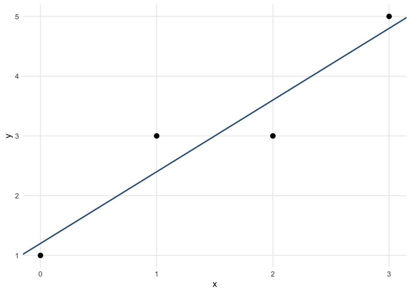
and the fitted regression line is
\[
\boxed{
\hat{Y}
=
1.2+1.2x.
}
\]
Step 4: Compute the Fitted Values
The fitted values are
\[
\hat{\mathbf{Y}}
=
\mathbf{X}\hat{\boldsymbol{\beta}}
=
\begin{pmatrix}
1.2\\
2.4\\
3.6\\
4.8
\end{pmatrix}.
\]
Step 5: Compute the Residuals
The residual vector is
\[\begin{align*}
\mathbf{e}
&=
\mathbf{Y}-\hat{\mathbf{Y}}\\
&=
\begin{pmatrix}
1\\
3\\
3\\
5
\end{pmatrix}
-
\begin{pmatrix}
1.2\\
2.4\\
3.6\\
4.8
\end{pmatrix}\\
&=
\begin{pmatrix}
-0.2\\
0.6\\
-0.6\\
0.2
\end{pmatrix}.
\end{align*}\]
Notice that
\[
\sum_{i=1}^4e_i
=
-0.2+0.6-0.6+0.2
=
0.
\]
This occurs because the model contains an intercept.
Step 6: Verify Orthogonality
We compute
\[
\mathbf{X}^\top\mathbf{e}
=
\begin{pmatrix}
1 & 1 & 1 & 1\\
0 & 1 & 2 & 3
\end{pmatrix}
\begin{pmatrix}
-0.2\\
0.6\\
-0.6\\
0.2
\end{pmatrix}
=
\begin{pmatrix}
0\\
0
\end{pmatrix}.
\]
Thus,
\[
\boxed{
\mathbf{X}^\top\mathbf{e}
=
\mathbf{0}.
}
\]
We can also verify that
\(\hat{\mathbf{Y}}^\top\mathbf{e}=0.\)
Step 7: Compute the Hat Matrix
The hat matrix is
\[
\mathbf{H}
=
\mathbf{X}
(\mathbf{X}^\top\mathbf{X})^{-1}
\mathbf{X}^\top.
\]
For this example,
\[
\mathbf{H}
=
\begin{pmatrix}
0.7 & 0.4 & 0.1 & -0.2\\
0.4 & 0.3 & 0.2 & 0.1\\
0.1 & 0.2 & 0.3 & 0.4\\
-0.2 & 0.1 & 0.4 & 0.7
\end{pmatrix}.
\]
Multiplying by \(\mathbf{Y}\) gives
\[
\mathbf{H}\mathbf{Y}
=
\begin{pmatrix}
1.2\\
2.4\\
3.6\\
4.8
\end{pmatrix}
=
\hat{\mathbf{Y}}.
\]
Thus, the hat matrix projects the observed response onto the model space.
We can verify the previous calculations in R.
<- c (0 , 1 , 2 , 3 )<- c (1 , 3 , 3 , 5 )<- data.frame (x = x,y = y<- lm (y ~ x, data = df)coef (fit)
The estimated coefficients are
\[
\hat{\beta}_0=1.2,
\qquad
\hat{\beta}_1=1.2.
\]
We can also compute the estimator directly using matrix operations.
  (Intercept) x
1           1 0
2           1 1
3           1 2
4           1 3
attr(,"assign")
[1] 0 1
<- matrix (y, ncol = 1 )<- solve (t (X) %*% X) %*% t (X) %*%
            [,1]
(Intercept)  1.2
x            1.2
Compute the fitted values and residuals:
<- X %*% beta_hat<- Y - y_hat
  [,1]
1  1.2
2  2.4
3  3.6
4  4.8
  [,1]
1 -0.2
2  0.6
3 -0.6
4  0.2
Check that the residuals sum to zero:
Compute the hat matrix:
<- %*% solve (t (X) %*% X) %*% t (X)round (H, 4 )
     1   2   3    4
1  0.7 0.4 0.1 -0.2
2  0.4 0.3 0.2  0.1
3  0.1 0.2 0.3  0.4
4 -0.2 0.1 0.4  0.7
Verify symmetry:
  1 2 3 4
1 0 0 0 0
2 0 0 0 0
3 0 0 0 0
4 0 0 0 0
Verify idempotence:
  1 2 3 4
1 0 0 0 0
2 0 0 0 0
3 0 0 0 0
4 0 0 0 0
Verify the normal equations geometrically:
Verify that fitted values and residuals are orthogonal:
round (t (y_hat) %*% e, 10 )
Construct the residual-maker matrix:
<- diag (nrow (X)) - Hround (M, 4 )
     1    2    3    4
1  0.3 -0.4 -0.1  0.2
2 -0.4  0.7 -0.2 -0.1
3 -0.1 -0.2  0.7 -0.4
4  0.2 -0.1 -0.4  0.3
  1 2 3 4
1 0 0 0 0
2 0 0 0 0
3 0 0 0 0
4 0 0 0 0
Verify that
\[
\mathbf{e}
=
\mathbf{M}\mathbf{Y}.
\]
Finally, plot the fitted regression line:
ggplot (df, aes (x, y)) + geom_point (size = 2.5 ) + geom_abline (intercept = coef (fit)[1 ], slope = coef (fit)[2 ],colour = "steelblue4" , linewidth = 0.8 ) + labs (x = "x" , y = "y" )
What Happens Without Full Column Rank?
Suppose
\[
\operatorname{rank}(\mathbf{X})
<
p.
\]
Then the columns of \(\mathbf{X}\) are linearly dependent, and
\[
\mathbf{X}^\top\mathbf{X}
\]
is singular.
Therefore,
\[
(\mathbf{X}^\top\mathbf{X})^{-1}
\]
does not exist.
When \(\mathbf{X}\) does not have full column rank,
a least squares solution still exists;
\(\hat{\boldsymbol{\beta}}\) may not be unique;the fitted vector \(\hat{\mathbf{Y}}\) is still unique;
the residual vector \(\mathbf{e}\) is still unique.
Thus,
\[
\boxed{
\hat{\boldsymbol{\beta}}
\text{ may not be unique, but }
\hat{\mathbf{Y}}
\text{ is unique.}
}
\]
The reason is geometric: even if several coefficient vectors represent the same point in \(\mathcal{C}(\mathbf{X})\) , the orthogonal projection of \(\mathbf{Y}\) onto \(\mathcal{C}(\mathbf{X})\) is unique.
We will discuss rank deficiency, generalized inverses, and estimability in more detail later.
Interpretation of the Geometry
The observed vector
\[
\mathbf{Y}
\in
\mathbb{R}^n.
\]
When \(\mathbf{X}\) has full column rank \(p\) , the model space
\[
\mathcal{C}(\mathbf{X})
\]
is a \(p\) -dimensional subspace of \(\mathbb{R}^n\) .
Least squares finds the point in this subspace that is closest to \(\mathbf{Y}\) .
The central relationships are
\[
\boxed{
\min_{\boldsymbol{\beta}}
\|
\mathbf{Y}-\mathbf{X}\boldsymbol{\beta}
\|_2^2
}
\]
\[
\Downarrow
\]
\[
\boxed{
\mathbf{X}^\top
(\mathbf{Y}-\mathbf{X}\hat{\boldsymbol{\beta}})
=
\mathbf{0}
}
\]
\[
\Downarrow
\]
\[
\boxed{
\mathbf{e}
\perp
\mathcal{C}(\mathbf{X})
}
\]
\[
\Downarrow
\]
\[
\boxed{
\hat{\mathbf{Y}}
=
\mathbf{H}\mathbf{Y}
}
\]
\[
\Downarrow
\]
\[
\boxed{
\mathbf{Y}
=
\hat{\mathbf{Y}}
+
\mathbf{e}.
}
\]
Thus,
fitted values are orthogonal projections;
residuals are orthogonal to the model space;
the hat matrix is a projection matrix;
the residual-maker matrix projects onto the orthogonal complement;
sum-of-squares decompositions are consequences of the Pythagorean theorem.
Looking Ahead: Statistical Properties of OLS
Everything we have done so far is primarily algebraic and geometric .
We defined \(\hat{\boldsymbol{\beta}}=(\mathbf{X}^\top\mathbf{X})^{-1}\mathbf{X}^\top\mathbf{Y}\) by solving an optimization problem.
However, under the statistical model, \(\mathbf{Y}=\mathbf{X}\boldsymbol{\beta}+\boldsymbol{\varepsilon},\) the response \(\mathbf{Y}\) is random. Therefore, \(\hat{\boldsymbol{\beta}}\) is also a random vector.
In Chapter 3 — Distribution Theory of OLS and Inference , we will study quantities such as
\[
\mathbb{E}
(\hat{\boldsymbol{\beta}}),\quad \text{and}\quad \operatorname{Var}
(\hat{\boldsymbol{\beta}}),
\] followed by estimation of \(\sigma^2\) , sampling distributions, confidence intervals, and hypothesis testing.
In this chapter, we introduced the least squares estimator through the optimization problem
\[
\hat{\boldsymbol{\beta}}
=
\arg\min_{\boldsymbol{\beta}}
\left\|
\mathbf{Y}
-
\mathbf{X}\boldsymbol{\beta}
\right\|_2^2.
\]
Differentiating the residual sum of squares leads to the normal equations
\[
\boxed{
\mathbf{X}^\top\mathbf{X}
\hat{\boldsymbol{\beta}}
=
\mathbf{X}^\top\mathbf{Y}.
}
\]
When \(\mathbf{X}\) has full column rank,
\[
\boxed{
\hat{\boldsymbol{\beta}}
=
(\mathbf{X}^\top\mathbf{X})^{-1}
\mathbf{X}^\top\mathbf{Y}.
}
\]
The fitted response is
\[
\hat{\mathbf{Y}}
=
\mathbf{H}\mathbf{Y},
\]
where
\[
\mathbf{H}
=
\mathbf{X}
(\mathbf{X}^\top\mathbf{X})^{-1}
\mathbf{X}^\top
\]
is the hat matrix.
Geometrically,
\[
\hat{\mathbf{Y}}
\]
is the orthogonal projection of \(\mathbf{Y}\) onto \(\mathcal{C}(\mathbf{X})\) .
The residual vector
\[
\mathbf{e}
=
\mathbf{Y}
-
\hat{\mathbf{Y}}
\]
lies in the orthogonal complement of the model space, so
\[
\mathbf{X}^\top\mathbf{e}
=
\mathbf{0}.
\]
Therefore,
\[
\boxed{
\mathbf{Y}
=
\hat{\mathbf{Y}}
+
\mathbf{e}
}
\]
is an orthogonal decomposition.
In Chapter 3 — Distribution Theory of OLS and Inference , we will treat \(\hat{\boldsymbol{\beta}}\) as a random vector and study its expectation, variance, sampling distribution, and the foundations of statistical inference for linear models.
Practice at Home
Explain why
\[
\mathbf{X}^\top\mathbf{e}
=
\mathbf{0}
\]
means that the residual vector is orthogonal to the column space \(\mathcal{C}(\mathbf{X})\) .
Explain why
\[
\hat{\mathbf{Y}}
=
\mathbf{H}\mathbf{Y}
\]
is an orthogonal projection, and why
\[
\mathbf{H}^2
=
\mathbf{H}.
\]
If the model contains an intercept, explain why
\[
\sum_{i=1}^n e_i
=
0
\]
and hence
\[
\bar{\hat{Y}}
=
\bar{Y}.
\]
Let
\[
\mathbf{X}
=
\begin{pmatrix}
1 & 0\\
1 & 1\\
1 & 2
\end{pmatrix},
\qquad
\mathbf{Y}
=
\begin{pmatrix}
1\\
2\\
2
\end{pmatrix}.
\]
Compute
\[
\hat{\boldsymbol{\beta}},
\qquad
\hat{\mathbf{Y}},
\qquad
\mathbf{e},
\]
and verify that
\[
\mathbf{X}^\top\mathbf{e}
=
\mathbf{0}.
\]
Show that the hat matrix
\[
\mathbf{H}
=
\mathbf{X}
(\mathbf{X}^\top\mathbf{X})^{-1}
\mathbf{X}^\top
\]
is symmetric and idempotent.
Side Fact: Matrix Calculus Facts Used in this chapter
Let \(\boldsymbol{\beta}\) be a column vector.
For a constant vector \(\mathbf{a}\) ,
\[
\frac{\partial}
{\partial\boldsymbol{\beta}}
\left(
\mathbf{a}^\top\boldsymbol{\beta}
\right)
=
\mathbf{a}.
\]
For a constant matrix \(\mathbf{A}\) ,
\[
\frac{\partial}
{\partial\boldsymbol{\beta}}
\left(
\boldsymbol{\beta}^\top
\mathbf{A}
\boldsymbol{\beta}
\right)
=
(\mathbf{A}+\mathbf{A}^\top)
\boldsymbol{\beta}.
\]
If \(\mathbf{A}\) is symmetric,
\[
\mathbf{A}^\top
=
\mathbf{A},
\]
and therefore
\[
\boxed{
\frac{\partial}
{\partial\boldsymbol{\beta}}
\left(
\boldsymbol{\beta}^\top
\mathbf{A}
\boldsymbol{\beta}
\right)
=
2\mathbf{A}\boldsymbol{\beta}.
}
\]
These identities justify the derivative used in the least squares criterion.