A belief function\(\mathrm{Be}(\cdot)\) is a function that assigns number to statements such that the large the number, the higher the degree of belief.
Let \(F, G\), and \(H\) be three possibly overlapping statements about the world.
For example:
F = { a person owns a smartphone }
G = { a person uses social media daily }
H = { a person works remotely at least part of the time }
or
F = { a person has a graduate degree }
G = { a person works in a STEM field }
H = { a person is employed in the private sector }
The perference over bets involving these statements can be used to define a belief function
\(\mathrm{Be}(F)>\mathrm{Be}(G)\) means you prefer a bet \(F\) is true over that \(G\) is true.
Also, we want \(\mathrm{Be}(\cdot)\) to describe our beliefs under certain conditions
\(\mathrm{Be}(F\mid H) > \mathrm{Be}(G\mid H)\) means that if we knew that \(H\) were true, then we would perfer to bet that \(F\) is also true over \(G\) is also true.
\(\mathrm{Be}(F\mid G) > \mathrm{Be}(F\mid H)\) means that if we bet on \(F\), we would perfer to do it under the condition that \(G\) is true rather than \(H\) is true.
Some more notations:
Let \(\neg\) denote negation. That is, \(\neg F\) is the statement that \(F\) is not true.
Let \(F \vee G\) denote the disjunction (or) of statements \(F\) and \(G\), meaning that at least one of \(F\) or \(G\) is true.
Let \(F \wedge G\) denote the conjunction (and) of statements \(F\) and \(G\), meaning that both \(F\) and \(G\) are true.
It has been argued by many that any function that is to numerically represent our beliefs should have the following properties:
B3: \(\mathrm{Be}(F \wedge G\mid H)\) can be derived from \(\mathrm{Be}(G\mid H)\) and \(\mathrm{Be}(F\mid G \wedge H)\).
How should we interpret these properties, and do they make sense?
B1 means that the number we assign to \(\mathrm{Be}(F \mid H)\), our conditional belief in \(F\) given \(H\), is bounded below and above by the numbers we assign to complete disbelief \(\mathrm{Be}(\neg H \mid H)\) and complete belief \(\mathrm{Be}(H \mid H)\).
B2 says that our belief that the truth lies in a given set of possibilities should not decrease as we add to the set of possibilities.
B3 is a bit trickier. To see why it makes sense, imagine you have to decide whether or not \(F\) and \(G\) are true, knowing that \(H\) is true. You could do this by first deciding whether or not \(G\) is true given \(H\), and if so, then deciding whether or not \(F\) is true given \(G\) and \(H\).
Recall the notation from (elementary) probability that, \(F\cup G\) means F or G, and \(F\cap G\) means F and G, and \(\emptyset\) is the empty set.
P2: \[\mathrm{Pr}(F \cup G \mid H)=\mathrm{Pr}(F \mid H)+\mathrm{Pr}(G \mid H),\quad \text{if}\quad F \cap G=\emptyset\]
P3: \[\mathrm{Pr}(F \cap G \mid H)=\mathrm{Pr}(G \mid H) \mathrm{Pr}(F \mid G \cap H)\]
2.1.1 Conclusion
You can see that, a probability function satisfy P1–P3 also satisfies B1–B3. Therefore, probability functions are a special case of belief functions, and we can use it to describe our belief.
2.2 Events, Partitions and Bayes’ Rule
A collectiion of sets \(\{H_1,\dots,H_K\}\) is a partition of another set \(\mathcal{H}\) if
\(H_i \cap H_j = \emptyset\) for all \(i \neq j\) (mutually exclusive);
In the context of indetifying which of several statements is true, if \(\mathcal{H}\) is the set of all possible truths and \(\{H_1,\dots,H_K\}\) is a partition of \(\mathcal{H}\), then exactly one set \(H_j\) contains the truth.
Let \(\mathcal{H}\) be the status of a statistical model.
Suppose \(\{H_1,\dots,H_K\}\) is a partition of \(\mathcal{H}\),\(\mathrm{Pr}(\mathcal{H})=1\) and \(E\) is some specific event. Then, by the axioms of probability, we have
Law of total probability \[
\sum_{k=1}^K \mathrm{Pr}(H_k)=\mathrm{Pr}\left(\bigcup_{k=1}^K H_k\right)=\mathrm{Pr}(\mathcal{H})=1
\]
Law of marginal probability \[
\mathrm{Pr}(E)=\sum_{k=1}^K \mathrm{Pr}(E \cap H_k)=\sum_{k=1}^K \mathrm{Pr}(E \mid H_k) \mathrm{Pr}(H_k)
\]
A subset of the 1996 General Social Survey includes data on the education level and income for a sample of males over 30 years of age. Let {H1,H2,H3,H4} be the events that a randomly selected person in this sample is in, respectively, the lower 25th percentile, the second 25th percentile, the third 25th percentile and the upper 25th percentile in terms of income. By definition,
Note that \(\{H1,H2,H3,H4\}\) is a partition and so these probabilities sum to 1. Let \(E\) be the event that a randomly sampled person from the survey has a college education. From the survey data, we have \[\{\mathrm{Pr}(E\mid H_1), \mathrm{Pr}(E\mid H_2),\mathrm{Pr}(E\mid H_3), \mathrm{Pr}(E\mid H_4)\} = \{.11, .19, .31, .53\}.\] These probabilities do not sum to 1 - they represent the proportions of people with college degrees in the four different income subpopulations \(H_1, H_2, H_3\) and \(H_4\). Now let’s consider the income distribution of the college-educated population. Using Bayes’ rule we can obtain
\(\{\mathrm{Pr}(H_1\mid E), \mathrm{Pr}(H_2\mid E), \mathrm{Pr}(H_3\mid E), \mathrm{Pr}(H_4 \mid E)\} = \{0.09, 0.17, 0.27, 0.47\} ,\) and we see that the income distribution for people in the college-educated population differs markedly from \(\{0.25, 0.25,0.25,0.25\}\), the distribution for the general population. Note that these probabilities do sum to 1 - they are the conditional probabilities of the events in the partition, given \(E\).
In Bayesian inference, \({H_1, . . . ,H_K}\) often refer to disjoint hypotheses or states of nature and \(E\) refers to the outcome of a survey, study or experiment. To compare hypotheses post-experimentally, we often calculate the following ratio: \[
\begin{aligned}
\frac{\operatorname{Pr}\left(H_i \mid E\right)}{\operatorname{Pr}\left(H_j \mid E\right)} & =\frac{\operatorname{Pr}\left(E \mid H_i\right) \operatorname{Pr}\left(H_i\right) / \operatorname{Pr}(E)}{\operatorname{Pr}\left(E \mid H_j\right) \operatorname{Pr}\left(H_j\right) / \operatorname{Pr}(E)} \\
& =\frac{\operatorname{Pr}\left(E \mid H_i\right) \operatorname{Pr}\left(H_i\right)}{\operatorname{Pr}\left(E \mid H_j\right) \operatorname{Pr}\left(H_j\right)} \\
& =\frac{\operatorname{Pr}\left(E \mid H_i\right)}{\operatorname{Pr}\left(E \mid H_j\right)} \times \frac{\operatorname{Pr}\left(H_i\right)}{\operatorname{Pr}\left(H_j\right)} \\
& =\text { "Bayes factor" × "prior beliefs". }
\end{aligned}
\] This calculation reminds us that Bayes’ rule does not determine what our beliefs should be after seeing the data, it only tells us how they should change after seeing the data.
2.3 Independence
Two events \(F\) and \(G\) are conditionally independent, if given \(H\), we have \(\mathrm{Pr}(F \cap G \mid H) = \mathrm{Pr}(F\mid H)\mathrm{Pr}(G\mid H)\).
How do we interpret conditional independence? By Axiom P3, the following is always true: \[
\begin{array}{rlll}
\operatorname{Pr}(G \mid H) \operatorname{Pr}(F \mid H \cap G) \stackrel{\text { always }}{=} \operatorname{Pr}(F \cap G \mid H) & \stackrel{\text { independence }}{=} \operatorname{Pr}(F \mid H) \operatorname{Pr}(G \mid H) \\
\operatorname{Pr}(G \mid H) \operatorname{Pr}(F \mid H \cap G) & = & \operatorname{Pr}(F \mid H) \operatorname{Pr}(G \mid H) \\
\operatorname{Pr}(F \mid H \cap G) & = & \operatorname{Pr}(F \mid H) .
\end{array}
\]
Thus, conditional independence implies that \(\mathrm{Pr}(F \mid H \cap G) = \mathrm{Pr}(F\mid H)\). In other words, if we know \(H\) is true, and \(F\) and \(G\) are conditionally independent given \(H\), then knowing \(G\) does not change our belief about \(F\).
Let’s consider the conditional dependence of \(F\) and \(G\) when \(H\) is assumed to be true in the following two situations:
Siutation 1:
F = { a hospital patient is a smoker }
G = { a hospital patient has lung cancer }
H = { smoking causes lung cancer}
Situation 2:
F = { a student studies regularly for an exam }
G = { a student receives a high exam score }
H = { studying improves exam performance }
Think: In both of these situations, H being true implies a relationship between \(F\) and \(G\). What about when \(H\) is not true?
2.4 Random Variables
In Bayesian inference a random variable is defined as an unknown numerical quantity about which we make probability statements. For example, the quantitative outcome of a survey, experiment or study is a random variable before the study is performed. Additionally, a fixed but unknown population parameter is also a random variable
2.4.1 Discrete Ramdon variables
Let \(Y\) be a random variable and let \(\mathcal{Y}\) be the set of all possible values that \(Y\) can take. If \(\mathcal{Y}\) is countable, meaning that \(\mathcal{Y} = \{y_1,y_2,\dots\}\), then \(Y\) is a discrete random variable.
The event that the outcome \(Y\) of our survey has the value \(Y\) is expressed as \(\{Y=y\}\). For each \(y\in\mathcal{Y}\), the shorthand notation for \(\mathrm{Pr}(Y=y)\) is \(p(y)\), and \(p(\cdot)\) is called the probability mass function of \(Y\), and with two properties
\(0 \leq p(y) \leq 1\) for all \(y\in\mathcal{Y}\),
\(\sum_{y\in\mathcal{Y}} p(y) = 1\).
General probability statements about \(Y\) can be derived from the pdf/pmf, for example, for any subset \(A \subseteq \mathcal{Y}\), we have \(\mathrm{Pr}(Y\in A) = \sum_{y\in A} p(y)\). When we have two disjoint subsets \(A\) and \(B\) of \(\mathcal{Y}\), we have \[\mathrm{Pr}(Y\in A \cup B) = \mathrm{Pr}(Y\in A) + \mathrm{Pr}(Y\in B)=\sum_{y\in A} p(y) + \sum_{y\in B} p(y).\]
Let \(Y\) be the number of successes in \(n\) independent Bernoulli trials, each with probability of success \(\theta\). Then, \(Y\) follows a Binomial distribution with parameters \(n\) and \(\theta\), denoted as \(Y \sim \mathrm{Binomial}(n,p)\). The probability mass function of \(Y\) is given by \[
p(y) = \mathrm{Pr}(Y=y) = \binom{n}{y} \theta^y (1-\theta)^{n-y}, \quad y=0,1,2,\dots,n.
\] If \(\theta=0.3\) and \(n=3\), then the probability of observing exactly 2 successes is \[
p(2) = \mathrm{Pr}(Y=2 \mid \theta=0.3) = \binom{3}{2
} (0.3)^2 (0.7)^{1} = 3 \cdot 0.09 \cdot 0.7 = 0.189.
\]
2.4.2 Continuous random variables
If \(\mathcal{Y}\) is uncountable, for example, \(\mathcal{Y} = \mathbb{R}\) or \(\mathcal{Y} = (0,1)\), then \(Y\) is a continuous random variable. In this case, we cannot list all possible values of \(Y\) and assign probabilities to each value. Instead, we use a probability distribution to describe the distribution of \(Y\). That is, the cummulative distribution function (cdf) defined as follows.
The cumulative distribution function (cdf) of a continuous random variable \(Y\) is defined as \[
F(y) = \mathrm{Pr}(Y \leq y), \quad y \in \mathcal{Y}.
\]
Note that, for the cdf \(F(y)\), we have the following properties:
\(0 \leq F(y) \leq 1\) for all \(y\in\mathcal{Y}\),
\(F(y)\) is non-decreasing, meaning that if \(y_1 < y_2\), then \(F(y_1) \leq F(y_2)\),
\(\lim_{y \to -\infty} F(y) = 0\)
\(\lim_{y \to \infty} F(y) = 1\).
Probability of various events can be derived from the cdf. For example, for any interval \(A = (a,b] \subseteq \mathcal{Y}\), we have \[
\mathrm{Pr}(Y \in A) = \mathrm{Pr}(a < Y \leq b) =
F(b) - F(a).
\] Also, \(\mathrm{Pr}(Y \leq a) = F(a)\) and \(\mathrm{Pr}(Y > a) = 1 - F(a)\).
2.4.3 Description of distributions through quantiles and moments
In this subsection, we discuss a few ways to describe probability distributions: quantiles and moments. They are used to describe the behaviour of the distribution compressing them into summary statistics.
The expectation or mean of a random variable \(Y\) can be thought as the centre of mass or the location of the distribution, which is defined as
For discrete random variable: \[
E(Y) = \sum_{y\in\mathcal{Y}} y p(y).
\]
For continuous random variable: \[
E(Y) = \int_{\mathcal{Y}} y f(y) dy.
\]
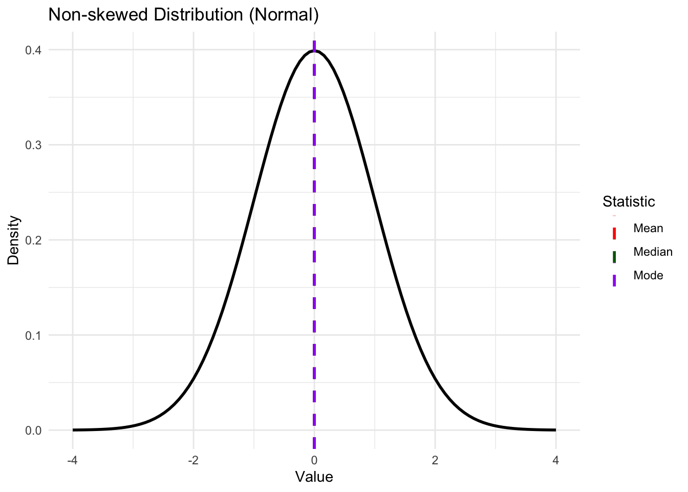
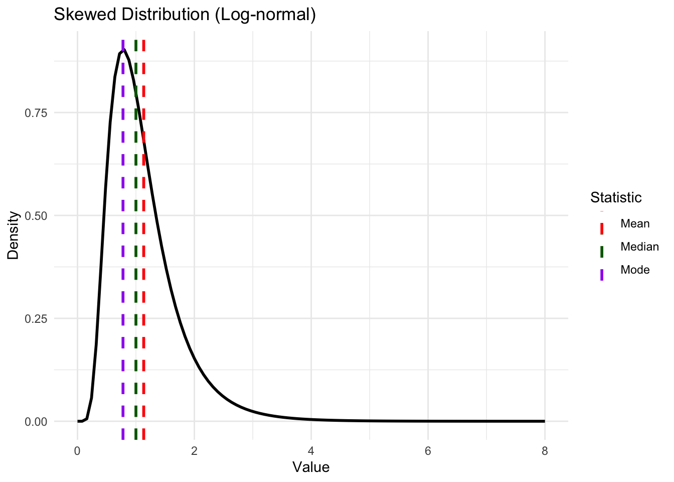
NoteDifference between mean, mode and median
Mean: the centre of mass of the distribution
Mode: The most probable value of \(Y\)
Median: The value of Y in the middle of the distribution.
In skewed distribution, the three will not equal to each other.
The mean is widely used in statistics and data analysis for several reasons:
Mathematical properties: The mean has desirable mathematical properties, such as linearity, which makes it easier to work with in various statistical analyses and models.
Sensitivity to all values: The mean takes into account all values in the dataset, providing a comprehensive measure of central tendency. It is also a scaled version of the total, which is often an interest
Foundation for other statistical measures: The mean serves as the basis for many other statistical measures, such as variance and standard deviation, which are essential for understanding the spread and variability of data.
Mean minimizes the sum of squared deviations: The mean is the value that minimizes the sum of squared deviations (i.e., the expected penalty by choosing one value) from itself, making it a natural choice for summarizing data.
May contains full information: In some distributions (e.g., bernoulli distribution), the mean contains all the information about the distribution, making it a sufficient statistic for inference.
The variance of a random variable \(Y\) measures the spread or dispersion of the distribution, and is defined as \[
\mathrm{Var}(Y) = E\left[(Y - E(Y))^2\right] = E[Y^2]- E^2[Y].
\] The standard deviation is the square root of the variance, denoted as \(\mathrm{SD}(Y) = \sqrt{\mathrm{Var}(Y)}\).
The quantile of order \(\alpha\) of a random variable \(Y\) is defined as the value \(y_\alpha\) such that \[
\mathrm{Pr}(Y \leq y_\alpha) = F(y_\alpha) = \alpha
\] for \(0 < \alpha < 1\).
For example, the median is the quantile of order 0.5, denoted as \(y_{0.5}\), which satisfies \(\mathrm{Pr}(Y \leq y_{0.5}) = 0.5\). Also, \((y_{0.025},y_{0.975})\) and \((y_{0.25},y_{0.75})\) contains 95% and 50% of the mass of the distribution, respectively.
2.5 Joint Disitrubiton
2.5.1 Discrete random variables
Let \(Y_1\) and \(Y_2\) be two random variables with possible values in \(\mathcal{Y}_1\) and \(\mathcal{Y}_2\), respectively. The joint distribution of \(Y_1\) and \(Y_2\) describes the probability of various combinations of values that \((Y_1,Y_2)\) can take.
Joint beliefs about \(Y_1\) and \(Y_2\) can be represented with probabilities. For example, for subsets \(A\subset \mathcal{Y}_1\) and \(B\subset \mathcal{Y}_2\), \(\mathrm{Pr}(\{Y_1\in A\} \cap \{Y_2 \in B\})\) represents our belief that \(Y_1\) takes a value in \(A\) and \(Y_2\) takes a value in \(B\). The joint pdf or joint density of \(Y_1\) and \(Y_2\) is defined as
The marginal density of \(Y_1\) can be computed from the joint density: \[
\begin{aligned}
p_{Y_1}\left(y_1\right) & \equiv \operatorname{Pr}\left(Y_1=y_1\right) \\
& =\sum_{y_2 \in \mathcal{Y}_2} \operatorname{Pr}\left(\left\{Y_1=y_1\right\} \cap\left\{Y_2=y_2\right\}\right) \\
& \equiv \sum_{y_2 \in \mathcal{Y}_2} p_{Y_1 Y_2}\left(y_1, y_2\right)
\end{aligned}
\]
The conditional density of \(Y_2\) given \(\{Y_1=y_1\}\) can be computed from the joint density and the marginal density: \[
\begin{aligned}
p_{Y_2 \mid Y_1}\left(y_2 \mid y_1\right) & =\frac{\operatorname{Pr}\left(\left\{Y_1=y_1\right\} \cap\left\{Y_2=y_2\right\}\right)}{\operatorname{Pr}\left(Y_1=y_1\right)} \\
& =\frac{p_{Y_1 Y_2}\left(y_1, y_2\right)}{p_{Y_1}\left(y_1\right)} .
\end{aligned}
\]
You should be able to see that
\(\left\{p_{Y_1}, p_{Y_2 \mid Y_1}\right\}\) can be derived from \(p_{Y_1 Y_2}\),
\(\left\{p_{Y_2}, p_{Y_1 \mid Y_2}\right\}\) can be derived from \(p_{Y_1 Y_2}\)
\(p_{Y_1 Y_2}\) can be derived from \(\left\{p_{Y_1}, p_{Y_2 \mid Y_1}\right\}\)
\(p_{Y_1 Y_2}\) can be derived from \(\left\{p_{Y_2}, p_{Y_1 \mid
Y_2}\right\}\)
BUT
\(p_{Y_1 Y_2}\) cannot be derived from \(\left\{p_{Y_1}, p_{Y_2}\right\}\).
The subscripts of density functions are often dropped, in which case the type of density function is determined by the arguments. For example,
\(p(y_1,y_2)=p_{Y_1 Y_2}(y_1,y_2)\) is the joint density of \(Y_1\) and \(Y_2\),
\(p(y_1)=p_{Y_1}(y_1)\) is the marginal density of \(Y_1\)
\(p(y_2 \mid y_1)=p_{Y_2\mid Y_1}(y_2 \mid y_1)\) is the conditional density of \(Y_2\) given \(\{Y_1=y_1\}\), and so on.
Suppose a sociological study reports the following joint distribution of parents’ education level and children’s income level in a population.
Joint distribution of education and income Suppose a sociological study reports the following joint distribution of parents’ education level and children’s income level in a population as shown in the Table below
Parent \ Child
Low Income
Middle Income
High Income
High School or Less
0.18
0.22
0.10
College
0.08
0.20
0.12
Graduate School
0.04
0.06
0.10
Suppose we randomly sample a parent–child pair from this population.
Let
- \(Y_1\) be the parent’s education level
- \(Y_2\) be the child’s income level
We are interested in the conditional probability that the child has high income, given that the parent has a college education.
We may answer this question using the conditional probability formula:
Thus, our conclusion from the table is, among children whose parents have a college education, 30% attain high income.
2.5.2 Continuous random variables
Let \(Y_1\) and \(Y_2\) be two continuous random variables with possible values in \(\mathcal{Y}_1\) and \(\mathcal{Y}_2\), respectively. The joint distribution of \(Y_1\) and \(Y_2\) describes the probability of various combinations of values that \((Y_1,Y_2)\) can take. We again work with the cumulative distribution function (cdf). The definition is given as follows.
Given a continuous joint cdf \(F_{Y_1 Y_2}(y_1,y_2)\), there is a function \(p_{Y_1,Y_2}\) such that \[
F_{Y_1,Y_2}(a,b) = \int_{-\infty}^a \int_{-\infty}^b p_{Y_1,Y_2}(y_1,y_2) dy_2 dy_1,
\] and \(p_{Y_1,Y_2}(y_1,y_2)\) is called the joint density function of \(Y_1\) and \(Y_2\).
Similar to the discrete case, we can derive marginal and conditional densities from the joint density as
Marginal density of \(Y_1\): \[
p_{Y_1}(y_1) = \int_{\mathcal{Y}_2} p_{Y_1,Y_2}(y_1,y_2) dy_2,
\]
Conditional density of \(Y_2\) given \(\{Y_1=y_1\}\): \[
p_{Y_2 \mid Y_1}(y_2 \mid y_1) = \frac{p_{Y_1,Y_2}(y_1,y_2)}{p_{Y_1}(y_1)}.
\]
Think about why \(p_{Y_2 \mid Y_1}(y_2 \mid y_1)\) is an actual pdf.
2.5.3 Mixed continuous and discrete variables
It is possible to have joint distributions involving both discrete and continuous random variables. For example, let \(Y_1\) be a discrete random variable taking values in \(\mathcal{Y}_1\) and \(Y_2\) be a continuous random variable taking values in \(\mathcal{Y}_2\). The joint distribution of \(Y_1\) and \(Y_2\) can be described by the joint density function \(p_{Y_1,Y_2}(y_1,y_2)\), which gives the probability that \(Y_1\) takes the value \(y_1\) and \(Y_2\) takes a value in an infinitesimal interval around \(y_2\). One such as example is that \(Y_1\) is a binary variable indicating the presence or absence of a disease, and \(Y_2\) is a continuous variable representing the severity of symptoms. Suppose we define
Marginal density \(p_{Y_1}\) from our belief \(\mathrm{Pr}(Y_1=y_1)\)
a conditional density \(p_{Y_2\mid Y_1}\) from \(\mathrm{Pr}(Y_2\le y_2\mid Y_1=y_1)\doteq F_{Y_2\mid Y_1}(y_2\mid y_1)\).
Then, the joint density can be derived as \[
p_{Y_1,Y_2}(y_1,y_2) = p_{Y_1}(y_1) p_{Y_2 \mid Y_1}(y_2 \mid y_1),
\] and the probability can be calculated as \[
\mathrm{Pr}(Y_1\in A,Y_2\in B) = \int_{y_2\in B} \left\{\sum_{y_1\in A}p_{Y_1,Y_2}(y_1,y_2)\right\}dy_2.
\]
2.5.4 Bayes’ rule and parameter estimation
Let
\(\theta\): proportion of people in a large population who have a certain charactersitic.
\(Y\): number of people in a small random sample from the population who have the charactersitic
Then, in this case, we may threat \(\theta\) as continuous random variable taking values in \(\Theta = (0,1)\), and \(Y\) as a discrete random variable taking values in \(\mathcal{Y}= \{0,1,2,\dots,n\}\), where \(n\) is the sample size. Bayesian estimation of the parameter\(\theta\) derives from the calculate of \(p(\theta\mid y)\) where \(y\) is the observed value of \(Y\). In Bayesian, this calculation first requires that we have a joint density \(p(y,\theta)\) representing our belief about \(\theta\) and the survey outcome \(Y\). Often, it is natural to construct this joint density from
\(p(\theta)\): our prior belief about \(\theta\) before seeing the data, and
\(p(y \mid \theta)\): belief about \(Y\) given \(\theta\), often called the likelihood function.
Once we observed \(\{Y=y\}\), we need to compute our updated belief about \(\theta\), represented by the posterior density\(p(\theta \mid y)\) as \[
p(\theta \mid y) = \frac{p(\theta,y)}{p(y)} = \frac{p(y \mid \theta) p(\theta)}{p(y)} = \frac{p(y \mid \theta) p(\theta)}{\int_{\Theta} p(y \mid \theta) p(\theta) d\theta}.
\]
If we have two values \(\theta_1\) and \(\theta_2\) in \(\Theta\) that may be true, then the ratio of their posterior densities is given by
From this calculation, we notice when we are calculating the relative posterior probability between two parameter values we do not need calculate \(p(y)\) out.
Another way to think about this is, for a function of \(\theta\), \[
p(\theta \mid y) \propto p(y \mid \theta) p(\theta).
\]
NoteNote
We will see that the numerator is the important part, while the denominator is just a normalizing constant to make sure the posterior density integrates to 1.
2.6 Independence Random Variables
Let \(Y_1,\dots,Y_n\) be random variables with joint density \(p(y_1,\dots,y_n)\), and \(\theta\) is the parameter describe the conditions under which the random variables are generated. We say that \(Y_1,\dots,Y_n\) are conditionally independent given \(\theta\) if every collection of \(n\) sets \(\{A_1,\dots,A_n\}\) satisfies \[
\mathrm{Pr}(Y_1 \in A_1,\dots,Y_n \in A_n \mid \theta) = \prod_{i=1}^n \mathrm{Pr}(Y_i \in A_i \mid \theta).
\] If we have independence property, then \[
\mathrm{Pr}(Y_i\in A_i \mid \theta, Y_j\in A_j) = \mathrm{Pr}(Y_i \in A_i \mid \theta),
\] so the conditional indpenddence can be interpreted as meaning that \(Y_j\) gives no additional information about \(Y_i\) once we know \(\theta\). Also, under independence, the joint density can be factorized as \[
p(y_1,\dots,y_n \mid \theta) = \prod_{i= 1}^n p_{Y_i}(y_i \mid \theta).
\]
If the samples are also identically distributed, meaning that each \(Y_i\) has the same marginal density \(p_Y(y \mid \theta)\), then the joint density can be further simplified as \[
p(y_1,\dots,y_n \mid \theta) = \prod_{i= 1}^n p_Y(y_i \mid \theta).
\]
In this case , we say that \(Y_1,\dots,Y_n\) are independent and identically distributed (i.i.d.) given \(\theta\), with notation \[
Y_1,\dots,Y_n\mid \theta \stackrel{i.i.d.}{\sim} p_Y(y \mid \theta).
\]
2.7 Exchangeability
A sequence of random variables \(Y_1,Y_2,\dots,Y_n\) is exchangeable if for any permutation \(\pi\) of the indices \(\{1,2,\dots ,n\}\), we have \[
p(y_1,y_2,\dots,y_n) = p(y_{\pi(1 )},y_{\pi(2)},\dots,y_{\pi(n)}).
\]
In other words, the joint density of an exchangeable sequence is invariant to the order of the random variables. That is, the labels contains no information about the outcome.
Suppose a factory produces a large batch of items. Each item may be either defective or non-defective.
Let \[
Y_i =
\begin{cases}
1, & \text{if the } i\text{th inspected item is defective}, \\
0, & \text{otherwise}.
\end{cases}
\]
We inspect \(n = 10\) items chosen at random from the batch and record \(Y_1, Y_2, \dots, Y_{10}.\)
Consider the following three observed sequences:
\(p(1,0,1,0,1,0,0,1,0,1)\)
\(p(0,1,0,1,0,1,1,0,0,1)\)
\(p(1,1,0,0,1,0,1,0,0,1)\)
Each sequence contains 5 defective items and 5 non-defective items.
Question: Is there a reason to assign these three sequences different probabilities?
If the inspection order conveys no additional information about quality, then only the number of defective items matters, not their positions in the sequence. This motivates the concept of exchangeability.
This probability depends only on the number of defective items, not their order.
Thus, we have exchangeability, even though the \(Y_i\) are not independent under this model of belief.
Conditional i.i.d. given a latent parameter implies marginal exchangeability. That is, if \(\theta \sim p(\theta)\) and \(Y_1,\dots,Y_n\) are conditionally i.i.d. given \(\theta\), then \(Y_1,\dots,Y_n\) (i.e., unconditional on \(\theta\)) are exchangeable.
For the Proof, see page 28 in Hopf (2009).
2.8 de Finetti’s Theorem
As of now, we have seen that conditional i.i.d. given a latent parameter implies marginal exchangeability. For example, \[
\begin{cases}
Y_1,\dots,Y_n \mid \theta \stackrel{i.i.d.}{\sim} \\
\theta \sim p(\theta) \end{cases} \implies Y_1,\dots,Y_n \text{ are exchangeable}.
\]
The converse is also true, as stated in de Finetti’s theorem.
Let \(Y_i\in\mathcal{Y}\) for all \(i \in\{1,2,\dots,n\}\) be an exchangeable sequence of random variables. Then, there exists a parameter space \(\Theta\) and a prior distribution \(p(\theta)\) on \(\Theta\) such that the joint distribution of \(Y_1,\dots,Y_n\) can be represented as \[
p(y_1,\dots,y_n) = \int_{\Theta} \left\{\prod_{i=1}^n p_Y(y_i \mid \theta)\right\} p(\theta) d\theta,
\] where \(p_Y(y \mid \theta)\) is a probability density function on \(\mathcal{Y}\) for each \(\theta \in \Theta\). The prior and sampling model depend on the form of the belief model \(p(y_1,\dots,y_n)\).
The probability distribution \(p(\theta)\) represents our belief about the outcomes \(\{Y_1,Y_2,\dots,Y_n\}\), induced by our belief model \(p(y_1,\dots,y_n)\). That is,
\(p(\theta)\) represents our belief about \(\lim_{n\to\infty} \sum Y_i/n\) in the binary sense
\(p(\theta)\) represents our belief about \(\lim_{n\to\infty} \sum (Y_i\le c)/n\) for each \(c\) in the general case.
The main idea of this and the previous section is as follows \[
\begin{aligned}
Y_1, \ldots, Y_n \mid \theta &\stackrel{\text{i.i.d.}}{\sim} p(\cdot \mid \theta), \\
\theta &\sim p(\theta)
\end{aligned}
\quad \Longleftrightarrow \quad
Y_1, \ldots, Y_n \text{ are exchangeable for all } n .
\]
Question: When is the condition of “exchangeability for all \(n\)” reasonable?
Have exchaneability and repeatability
Exchangeability holds if the labels convey no information
repeatability hold includes the follows
\(Y_1,\dots,Y_n\) are outcomes of a repeartable experiment
\(Y_1,\dots,Y_n\) are sampled from a finite population with replacement
\(Y_1,\dots,Y_n\) are sampled from an infinite population without replacement.
NoteIn large finite population
Note, if \(Y_1,\dots,Y_n\) are exchangeable and sampled from a finite population of size \(N\) that is way bigger than \(n\) without replacement, then they can be modelled as approximate being conditional i.i.d.
This Chapter follows closely with Chapter 2 in Hoff (2009).