8 Appendix: Introduction to JAGS and BUGS language

8.1 Why learn JAGS?

So far, we have written Monte Carlo and Gibbs samplers directly in R. This is useful for understanding the mechanics of Bayesian computation, but it becomes inconvenient when models are more complicated.

JAGS stands for Just Another Gibbs Sampler. It is a program for fitting Bayesian hierarchical models using MCMC, especially Gibbs sampling and related methods.

JAGS uses the BUGS language, where BUGS stands for Bayesian inference Using Gibbs Sampling.

The basic idea is simple:

we describe the statistical model in BUGS syntax;
we provide the observed data;
we choose which parameters to monitor;
JAGS runs the MCMC algorithm and returns posterior samples.

8.2 What BUGS language does

BUGS language is a model specification language. It is not a general programming language like R or Python.

Its role is to describe:

the sampling model
the prior distributions
deterministic relationships among parameters
optional derived quantities

For example:

\[ Y_i \mid \theta \sim \text{Poisson}(\theta), \qquad \theta \sim \text{Gamma}(a,b) \]

Instead of writing the Gibbs sampler ourselves, we simply describe the model and JAGS handles the sampling.

8.3 History

BUGS was developed in the 1990s by David Spiegelhalter and colleagues at the University of Cambridge.
JAGS was created by Martyn Plummer in the early 2000s as a more flexible and open-source alternative to BUGS.
Both BUGS and JAGS have been widely used in academia and industry for Bayesian data analysis, especially in fields like ecology, epidemiology, and social sciences.
JAGS is designed to be compatible with BUGS models, so most BUGS code can be run in JAGS with little or no modification.
JAGS is often used in conjunction with R through packages like rjags and jagsUI, which provide an interface for running JAGS models from R.
The BUGS language has influenced the development of other probabilistic programming languages, such as Stan, nimble and PyMC3, which also allow users to specify Bayesian models in a high-level syntax.
JAGS continues to be maintained and updated, with the latest version being 4.3.2 as of 2026.
coda package is often used to analyze MCMC output from JAGS, providing tools for convergence diagnostics and posterior summaries.

8.4 Basic structure of a JAGS model

A JAGS model is written inside a model {} block.

model {
  for (i in 1:n) {
    y[i] ~ dpois(theta)
  }

  theta ~ dgamma(a, b)
}

The first part describes the likelihood, and the second part specifies the prior.

8.5 BUGS syntax rules

Stochastic nodes

Random variables are written using ~.

theta ~ dgamma(a, b)
y[i] ~ dpois(theta)

Deterministic nodes

Deterministic relationships use <-.

sigma <- 1 / sqrt(tau)
mu[i] <- alpha + beta * x[i]

Loops

Repeated data are handled with loops.

for (i in 1:n) {
  y[i] ~ dnorm(mu, tau)
}

Comments

Use # for comments.

# prior distribution
theta ~ dnorm(0, 0.01)

JAGS syntax

Pay attention to the JAGS syntax. Sometimes it may be different from what you expect! For instance, JAGS uses precision rather than variance for normal distributions dnorm(mean, precision). Precision is

\[ \tau = \frac{1}{\sigma^2}. \]

or in the lecture, we used \(\tilde{\sigma}^2=1/\sigma^2\).

In R code, we write

tau <- 1 / sigma^2

Common probability distributions in JAGS (BUGS language)
Distribution	JAGS syntax
Normal	`dnorm(mu, tau)`
Poisson	`dpois(lambda)`
Binomial	`dbin(p, n)`
Bernoulli	`dbern(p)`
Gamma	`dgamma(a, b)`
Beta	`dbeta(a, b)`
Uniform	`dunif(a, b)`

8.6 Example: Beta–Binomial model

\[ Y \mid \theta \sim \text{Binomial}(n,\theta), \qquad \theta \sim \text{Beta}(a,b) \]

JAGS model:

model {
  y ~ dbin(theta, n)
  theta ~ dbeta(a, b)
}

For multiple observations:

model {
  for (i in 1:n) {
    y[i] ~ dbern(theta)
  }
  theta ~ dbeta(a, b)
}

\[ Y_i \mid \theta \sim \text{Poisson}(\theta), \qquad \theta \sim \text{Gamma}(a,b) \]

JAGS:

model {
  for (i in 1:n) {
    y[i] ~ dpois(theta)
  }

  theta ~ dgamma(a, b)
}

\[ Y_i \mid \theta,\tau \sim \text{Normal}(\theta,\tau) \]

Priors

\[ \theta \sim \text{Normal}(\mu_0,\tau_0), \qquad \tau \sim \text{Gamma}(a,b) \]

JAGS model:

model {
  for (i in 1:n) {
    y[i] ~ dnorm(theta, tau)
  }

  theta ~ dnorm(mu0, tau0)
  tau ~ dgamma(a, b)

  sigma <- 1 / sqrt(tau)
}

8.7 Data list in R

data_jags <- list(
  y = y,
  n = length(y),
  a = 2,
  b = 1
)

8.8 Parameters to monitor

params <- c("theta")

8.9 Example JAGS workflow

library(jagsUI)

fit <- jags(
  data = data_jags,
  parameters.to.save = params,
  model.file = textConnection(model_string),
  n.chains = 3,
  n.iter = 5000,
  n.burnin = 1000
)

print(fit)

Initial values

Optional but sometimes useful.

inits <- function() {
  list(theta = 1)
}

Posterior output

Typical outputs include

posterior means
credible intervals
trace plots
density plots
effective sample size
\(\hat{R}\) convergence diagnostic

Useful functions in the BUGS/JAGS language
Function	Meaning
`log(x)`	logarithm
`exp(x)`	exponential
`sqrt(x)`	square root
`pow(x, a)`	power
`step(x)`	indicator function

Example:

tau <- pow(sigma, -2)

8.10 Indexing

Sometimes, for each of the data \(y_i\), you may want to have a different prior mean \(\mu_i\) that depends on covariates \(x_i\). This can be done as follows

for (i in 1:n) {
  y[i] ~ dnorm(mu[i], tau)
  mu[i] <- alpha + beta * x[i]
}

In this section we fit a simple Bayesian Poisson model in JAGS. Suppose

\[ Y_1,\ldots,Y_n \mid \theta \sim \text{i.i.d. Poisson}(\theta), \]

with prior

\[ \theta \sim \text{Gamma}(a,b), \]

where the Gamma distribution is parameterized by shape \(a\) and rate \(b\).

We will:

specify the model in BUGS/JAGS language;
prepare the data in R;
run JAGS using jagsUI;
extract posterior samples;
compare the MCMC output with the exact posterior.

8.10.1 Data

We use the following toy dataset:

y <- c(3, 2, 4, 1, 3)
n <- length(y)

a <- 2
b <- 1
sum_y <- sum(y)

y

[1] 3 2 4 1 3

sum_y

[1] 13

Under the Poisson–Gamma model, the posterior distribution is available analytically:

\[ \theta \mid y \sim \text{Gamma}!\left(a+\sum_{i=1}^n y_i,; b+n\right). \]

So in this example,

\[ \theta \mid y \sim \text{Gamma}(2+13,;1+5)=\text{Gamma}(15,6). \]

This makes the example useful because we can compare the JAGS output to the exact answer.

Step 1: write the JAGS model

In BUGS language, the model is

model_string <- "
model {

  # likelihood
  for (i in 1:n) {
    y[i] ~ dpois(theta)
  }

  # prior
  theta ~ dgamma(a, b)

}
"
cat(model_string)


model {

  # likelihood
  for (i in 1:n) {
    y[i] ~ dpois(theta)
  }

  # prior
  theta ~ dgamma(a, b)

}

A few notes:

dpois(theta) means Poisson with mean \(\theta\);
dgamma(a, b) in JAGS uses shape and rate;
theta is the parameter we want to estimate.

Step 2: prepare the data and monitored parameters

JAGS needs the data in a named list

data_jags <- list(
  y = y,
  n = n,
  a = a,
  b = b
)

params <- c("theta")

We will monitor only theta.

Step 3: choose initial values

Initial values are optional here, but we include them for completeness.

inits <- function() {
  list(theta = 2)
}

Step 4: run JAGS

library(jagsUI)

set.seed(8310)

fit <- jags(
  data = data_jags,
  inits = inits,
  parameters.to.save = params,
  model.file = textConnection(model_string),
  n.chains = 3,
  n.iter = 5000,
  n.burnin = 1000,
  n.thin = 2
)


Processing function input....... 

Done. 
 
Compiling model graph
   Resolving undeclared variables
   Allocating nodes
Graph information:
   Observed stochastic nodes: 5
   Unobserved stochastic nodes: 1
   Total graph size: 9

Initializing model

Adaptive phase..... 
Adaptive phase complete 
 

 Burn-in phase, 1000 iterations x 3 chains 
 

Sampling from joint posterior, 4000 iterations x 3 chains 
 

Calculating statistics....... 

Done.

Now print the summary:

print(fit)

JAGS output for model '4', generated by jagsUI.
Estimates based on 3 chains of 5000 iterations,
adaptation = 100 iterations (sufficient),
burn-in = 1000 iterations and thin rate = 2,
yielding 6000 total samples from the joint posterior. 
MCMC ran for 0 minutes at time 2026-03-15 14:42:30.281138.

           mean    sd   2.5%    50%  97.5% overlap0 f Rhat n.eff
theta     2.491 0.642  1.411  2.435  3.902    FALSE 1    1  6000
deviance 16.957 1.247 16.067 16.481 20.584    FALSE 1    1  6000

Successful convergence based on Rhat values (all < 1.1). 
Rhat is the potential scale reduction factor (at convergence, Rhat=1). 
For each parameter, n.eff is a crude measure of effective sample size. 

overlap0 checks if 0 falls in the parameter's 95% credible interval.
f is the proportion of the posterior with the same sign as the mean;
i.e., our confidence that the parameter is positive or negative.

DIC info: (pD = var(deviance)/2) 
pD = 0.8 and DIC = 17.734 
DIC is an estimate of expected predictive error (lower is better).

This output includes posterior means, standard deviations, credible intervals, and convergence diagnostics.

Step 5: compare with the exact posterior

The exact posterior is

\[ \theta \mid y \sim \text{Gamma}(15,6). \]

So the exact posterior mean is

\[ E(\theta \mid y) = \frac{15}{6} = 2.5. \]

The exact posterior variance is

\[ \mathrm{Var}(\theta \mid y) = \frac{15}{6^2} = \frac{15}{36}. \]

We can compute the exact summaries in R:

shape_post <- a + sum_y
rate_post  <- b + n

exact_mean <- shape_post / rate_post
exact_var  <- shape_post / rate_post^2
exact_ci   <- qgamma(c(0.025, 0.975), shape = shape_post, rate = rate_post)

exact_mean

[1] 2.5

exact_var

[1] 0.4166667

exact_ci

[1] 1.399231 3.914937

The JAGS summary for theta should be very close to these values.

Step 6: extract posterior samples

The posterior samples are stored inside the fitted object.

theta_post <- fit$samples[, , "theta"]
theta_post <- as.vector(theta_post)

head(theta_post)

[[1]]
Markov Chain Monte Carlo (MCMC) output:
Start = 1002 
End = 1014 
Thinning interval = 2 
        theta deviance
[1,] 1.560872 18.94180
[2,] 2.548968 16.07122
[3,] 3.785898 18.15506
[4,] 2.465718 16.10206
[5,] 2.216374 16.38049
[6,] 2.061858 16.71422
[7,] 2.080451 16.66675

[[2]]
Markov Chain Monte Carlo (MCMC) output:
Start = 1002 
End = 1014 
Thinning interval = 2 
        theta deviance
[1,] 2.597255 16.06616
[2,] 2.152139 16.50281
[3,] 2.207936 16.39529
[4,] 2.923875 16.25254
[5,] 2.964158 16.29960
[6,] 2.286347 16.27207
[7,] 3.593582 17.58737

[[3]]
Markov Chain Monte Carlo (MCMC) output:
Start = 1002 
End = 1014 
Thinning interval = 2 
        theta deviance
[1,] 1.738204 17.91732
[2,] 2.491540 16.08941
[3,] 2.296215 16.25878
[4,] 1.960389 17.01161
[5,] 2.444164 16.11480
[6,] 3.173188 16.61816
[7,] 3.100759 16.49421

attr(,"class")
[1] "mcmc.list"

length(theta_post)

[1] 3

These are MCMC draws from the posterior distribution of \(\theta\).

Step 7: posterior histogram and exact density

Now compare the JAGS samples to the exact Gamma posterior density.

library(ggplot2)
theta_post <- as.numeric(as.matrix(fit$samples)[,"theta"])

theta_df <- data.frame(theta = theta_post)
ggplot(theta_df, aes(x = theta)) +
  geom_histogram(aes(y = after_stat(density)),
                 bins = 30,
                 fill = "grey80",
                 color = "white") +
  stat_function(
    fun = dgamma,
    args = list(shape = shape_post, rate = rate_post),
    linewidth = 1.2,
    color = "black"
  ) +
  labs(
    title = "Posterior of theta: JAGS samples vs exact density",
    x = expression(theta),
    y = "Density"
  ) +
  theme_minimal()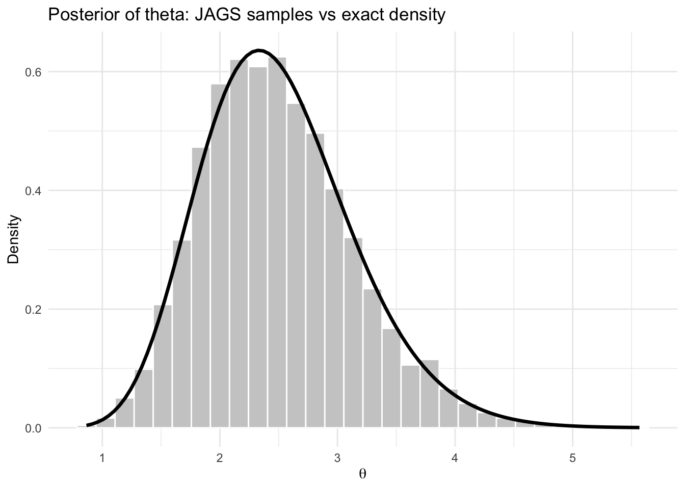

The histogram of the JAGS samples should align closely with the exact posterior density.

Step 8: posterior probability of an event

Suppose we want to estimate

\[ \Pr(\theta < 2.8 \mid y). \]

From the JAGS samples:

mean(theta_post < 2.8)

[1] 0.7071667

From the exact posterior:

pgamma(2.8, shape = shape_post, rate = rate_post)

[1] 0.702895

These two values should be close.

Step 9: posterior predictive simulation

Suppose \(\tilde Y\) is a future observation from the same population. The posterior predictive distribution is

\[ p(\tilde y \mid y) ＝ \int p(\tilde y \mid \theta),p(\theta \mid y),d\theta. \]

Using the JAGS samples, we can simulate from the posterior predictive distribution:

set.seed(8310)
y_tilde <- rpois(length(theta_post), lambda = theta_post)

head(y_tilde)

[1] 1 3 2 2 1 1

mean(y_tilde)

[1] 2.486

var(y_tilde)

[1] 2.957964

hist(y_tilde,
     breaks = seq(-0.5, max(y_tilde) + 0.5, by = 1),
     col = "grey85",
     border = "white",
     main = "Posterior predictive distribution",
     xlab = expression(tilde(Y)))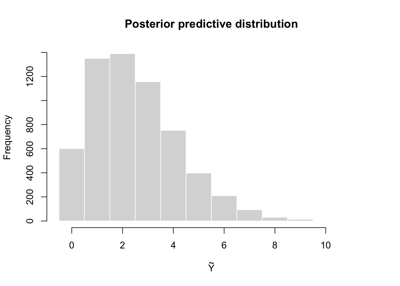

This histogram represents the distribution of a future observation \(\tilde Y\) given the observed data \(y\).

Interpretation

This example illustrates the full JAGS workflow:

specify a Bayesian model in BUGS language;
provide the data and priors;
run MCMC in JAGS;
summarize the posterior;
compare with an exact answer when available.

Because the Poisson–Gamma model is conjugate, this example is especially useful for learning. The JAGS output should agree closely with the exact posterior

\[ \text{Gamma}(15,6). \]

Full code in one chunk

library(jagsUI)
library(coda)
library(ggplot2)

# ===============================
# Data
# ===============================
y <- c(3, 2, 4, 1, 3)
n <- length(y)
a <- 2
b <- 1
sum_y <- sum(y)

# ===============================
# JAGS model
# ===============================
model_string <- "
model {

  for (i in 1:n) {
    y[i] ~ dpois(theta)
  }

  theta ~ dgamma(a, b)

}
"

# ===============================
# Data list for JAGS
# ===============================
data_jags <- list(
  y = y,
  n = n,
  a = a,
  b = b
)

params <- c("theta")

inits <- function() {
  list(theta = 2)
}

# ===============================
# Run JAGS
# ===============================
set.seed(8310)

fit <- jags(
  data = data_jags,
  inits = inits,
  parameters.to.save = params,
  model.file = textConnection(model_string),
  n.chains = 3,
  n.iter = 5000,
  n.burnin = 1000,
  n.thin = 2
)


Processing function input....... 

Done. 
 
Compiling model graph
   Resolving undeclared variables
   Allocating nodes
Graph information:
   Observed stochastic nodes: 5
   Unobserved stochastic nodes: 1
   Total graph size: 9

Initializing model

Adaptive phase..... 
Adaptive phase complete 
 

 Burn-in phase, 1000 iterations x 3 chains 
 

Sampling from joint posterior, 4000 iterations x 3 chains 
 

Calculating statistics....... 

Done.

print(fit)

JAGS output for model '4', generated by jagsUI.
Estimates based on 3 chains of 5000 iterations,
adaptation = 100 iterations (sufficient),
burn-in = 1000 iterations and thin rate = 2,
yielding 6000 total samples from the joint posterior. 
MCMC ran for 0 minutes at time 2026-03-15 14:35:57.462946.

           mean    sd   2.5%    50%  97.5% overlap0 f Rhat n.eff
theta     2.491 0.642  1.411  2.435  3.902    FALSE 1    1  6000
deviance 16.957 1.247 16.067 16.481 20.584    FALSE 1    1  6000

Successful convergence based on Rhat values (all < 1.1). 
Rhat is the potential scale reduction factor (at convergence, Rhat=1). 
For each parameter, n.eff is a crude measure of effective sample size. 

overlap0 checks if 0 falls in the parameter's 95% credible interval.
f is the proportion of the posterior with the same sign as the mean;
i.e., our confidence that the parameter is positive or negative.

DIC info: (pD = var(deviance)/2) 
pD = 0.8 and DIC = 17.734 
DIC is an estimate of expected predictive error (lower is better).

# ===============================
# Exact posterior
# ===============================
shape_post <- a + sum_y
rate_post  <- b + n

exact_mean <- shape_post / rate_post
exact_var  <- shape_post / rate_post^2
exact_ci   <- qgamma(c(0.025,0.975), shape = shape_post, rate = rate_post)

exact_mean

[1] 2.5

exact_var

[1] 0.4166667

exact_ci

[1] 1.399231 3.914937

# ===============================
# Extract posterior samples
# ===============================
theta_post <- as.numeric(as.matrix(fit$samples)[,"theta"])

theta_df <- data.frame(theta = theta_post)

# ===============================
# Posterior distribution plot
# ===============================
ggplot(theta_df, aes(x = theta)) +
  geom_histogram(aes(y = after_stat(density)),
                 bins = 30,
                 fill = "grey80",
                 color = "white") +
  stat_function(
    fun = dgamma,
    args = list(shape = shape_post, rate = rate_post),
    linewidth = 1.2,
    color = "black"
  ) +
  labs(
    title = "Posterior of theta: JAGS samples vs exact density",
    x = expression(theta),
    y = "Density"
  ) +
  theme_minimal()

# ===============================
# Posterior probability example
# ===============================
mean(theta_post < 2.8)

[1] 0.7071667

pgamma(2.8, shape = shape_post, rate = rate_post)

[1] 0.702895

# ===============================
# Posterior predictive simulation
# ===============================
set.seed(8310)

y_tilde <- rpois(length(theta_post), lambda = theta_post)

pred_df <- data.frame(y_tilde = y_tilde)

# ===============================
# Posterior predictive plot
# ===============================
ggplot(pred_df, aes(x = y_tilde)) +
  geom_histogram(
    binwidth = 1,
    fill = "grey80",
    color = "white",
    boundary = -0.5
  ) +
  labs(
    title = "Posterior Predictive Distribution",
    x = expression(tilde(Y)),
    y = "Count"
  ) +
  theme_minimal()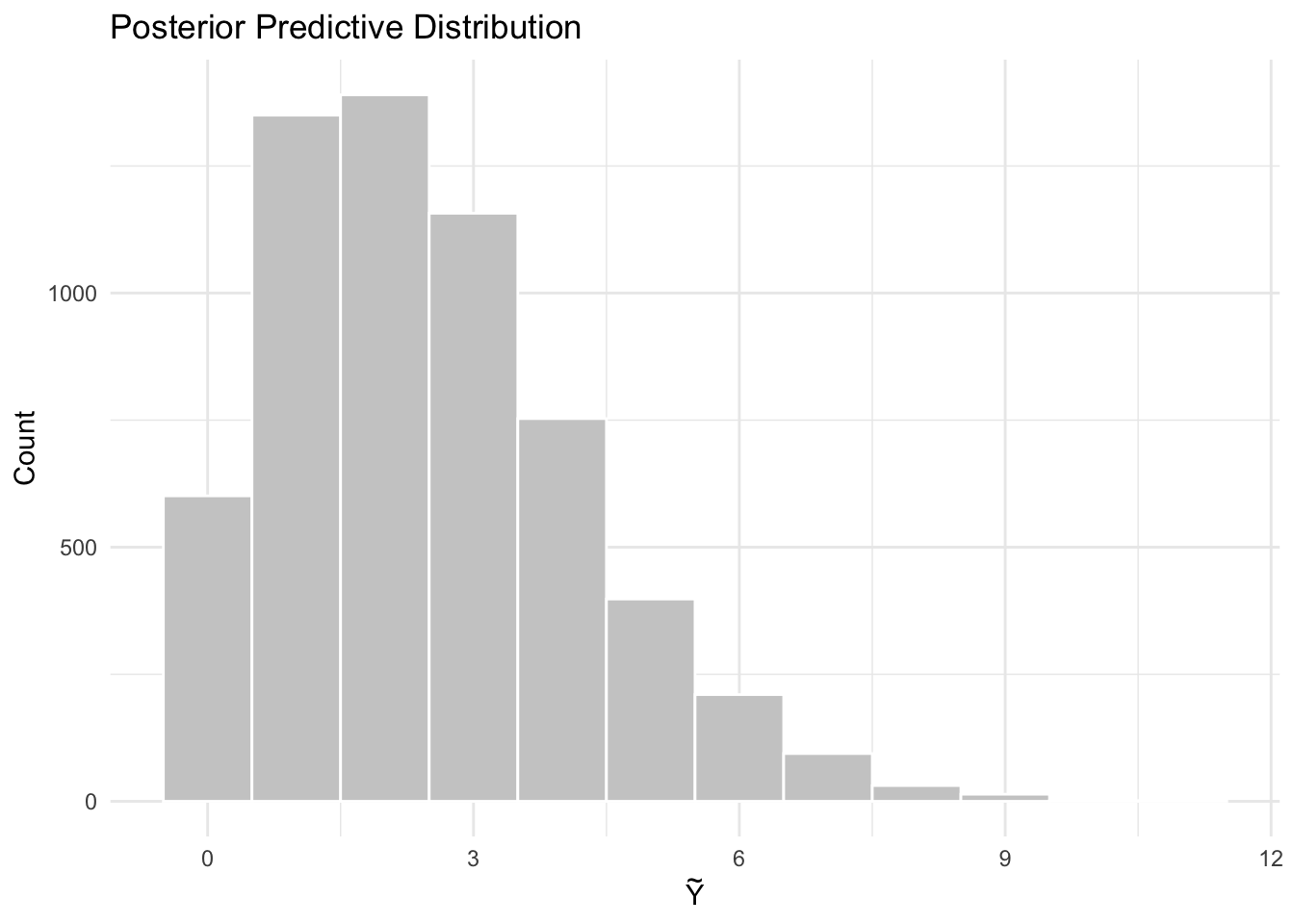

8.11 Summary and Take home message

JAGS performs Bayesian inference using MCMC.
Models are written in the BUGS language.
~ denotes a distribution.
<- denotes deterministic relationships.
Normal distributions use precision instead of variance.
JAGS separates model, data, and parameters.

Common (beginner) mistakes

Forgetting that normal uses precision
Mixing deterministic <- and stochastic ~
Assuming all R syntax works inside JAGS
Forgetting to pass constants in the data list

Reference: