3 Bayesian Inference for single parameter models

Leading objectives:

Understand how to perform Bayesian inference on a single parameter model.

Binomial model with given n

Poission model

Exponential family

Recall the important ingredients of Bayesian inference:

Prior distribution: \(\pi(\theta)\)
Likelihood function: \(p(y \mid \theta)\)
Posterior distribution: \(p(\theta \mid y) \propto p(y \mid \theta) \pi(\theta)\)

3.1 Three basic ingredients of Bayesian inference

3.1.1 Prior

The prior distribution encodes our beliefs about the parameter \(\theta\) before conduct any experiments.

Prior and Data are independent

Note that, the prior distribution is independent of the data. It represents our knowledge or beliefs about the parameter before seeing the data.

How do we choose a prior?

Informative priors: Based on previous studies or expert knowledge
Weakly informative priors: Provide some regularization without dominating the data
Non-informative priors: Attempt to be “objective” (e.g., uniform, Jeffreys prior)

3.1.2 Likelihood

The likelihood function represents the probability of observing the data given the parameter \(\theta\). It can be derived from the assumed statistical model for the data or experiment, i.e., \(y \sim p(y \mid \theta)\), or we can estimate this non-parametrically (i.e., without assuming the underlying distribution is the one we know.).

Likelihood is NOT a probability distribution for \(\theta\)

Note that, the likelihood function is not a probability distribution for \(\theta\) itself. It is a function of \(\theta\) for fixed data \(y\).

3.1.3 Posterior

The posterior distribution combines the prior and likelihood to update our beliefs about \(\theta\) after observing the data. It is given by Bayes’ theorem: \[ p(\theta \mid y) = \frac{p(y \mid \theta) \pi(\theta)}{p(y)}, \] where \(p(y) = \int p(y \mid \theta) \pi(\theta) d\theta\) is the marginal likelihood or evidence.

3.1.4 An simple example

Examples:

Beta prior + Binomial likelihood → Beta posterior
Normal prior + Normal likelihood (known variance) → Normal posterior
Gamma prior + Poisson likelihood → Gamma posterior

Advantages: - Analytical posteriors (no numerical integration needed) - Interpretable parameters - Computationally efficient

Limitations:

May not reflect true prior beliefs
Modern computing makes non-conjugate priors feasible

Let’s look a simple example to illustrate the convenience of conjugate priors. Consider a Binomial model with unknown success probability \(\theta\) and known number of trials \(n\). We can use a Beta prior for \(\theta\).

Suppose we have a Binomial model with known number of trials \(n\) and unknown success probability \(\theta\). We can use a Beta prior for \(\theta\).

Prior: \(\theta \sim \text{Beta}(\alpha, \beta)\)
Likelihood: \(y \mid \theta \sim \text{Binomial}(n, \theta)\)

The derivation of the posterior is as follows:

\[ \begin{aligned} p(y \mid \theta) & = \binom{n}{y} \theta^y (1 - \theta)^{n - y}, \\ \pi(\theta) & = \frac{\theta^{\alpha - 1} (1 - \theta)^{\beta - 1}}{B(\alpha, \beta)}, \end{aligned} \] where \(B(\alpha, \beta)\) is the Beta function. Then the posterior is proportional to: \[ p(\theta \mid y) \propto p(y \mid \theta) \pi(\theta) \propto \theta^{y + \alpha - 1} (1 - \theta)^{n - y + \beta - 1}. \] This is the kernel of a Beta distribution with parameters \((\alpha + y, \beta + n - y)\). Thus, the posterior distribution is: \[ \theta \mid y \sim \text{Beta}(\alpha + y, \beta + n - y). \]

Thus, the Posterior is \(\theta \mid y \sim \text{Beta}(\alpha + y, \beta + n - y)\).

3.2 Happiness Data – the first example of Bayesian inference procedure

We study Bayesian inference for a binomial proportion \(\theta\) when the sample size \(n\) is fixed. In this example, we want to see what is the procedure of doing Bayesian inference

In the 1998 General Social Survey, each female respondent aged 65 or over was asked whether she was generally happy.

Define the response variable \[ Y_i = \begin{cases} 1, & \text{if respondent } i \text{ reports being generally happy},\\ 0, & \text{otherwise}, \end{cases} \qquad i = 1,\ldots,n, \] where \(n = 129\).

Because we lack information that distinguishes individuals, it is reasonable to treat the responses as exchangeable.
That is, before observing the data, the labels or ordering of respondents carry no information.

Since the sample size \(n\) is small relative to the population size \(N\) of senior women, results from the previous chapter justify the following modeling approximation.

Modeling Assumptions: Our beliefs about \((Y_1,\ldots,Y_{129})\) are described by:

An unknown population proportion \[ \theta = \frac{1}{N}\sum_{i=1}^N Y_i, \] where \(\theta\) represents the proportion of generally happy individuals in the population.
A sampling model given \(\theta\)

Conditional on \(\theta\), the responses \(Y_1,\ldots,Y_{129}\) are independent and identically distributed Bernoulli random variables with \[ \Pr(Y_i = 1 \mid \theta) = \theta. \]

Given the population proportion \(\theta\), each respondent independently reports being happy with probability \(\theta\).

Likelihood: Under this model, the probability of observing data \(\{y_1,\ldots,y_{129}\}\) given \(\theta\) is \[ p(y_1,\ldots,y_{129} \mid \theta) = \theta^{\sum_{i=1}^{129} y_i} (1-\theta)^{129-\sum_{i=1}^{129} y_i}. \]

This expression depends on the data only through the sufficient statistic \[ S = \sum_{i=1}^{129} Y_i, \] the total number of respondents who report being generally happy.

For the happiness data, \[ S = 118, \] so the likelihood simplifies to \[ p(y_1,\ldots,y_{129} \mid \theta) = \theta^{118}(1-\theta)^{11}. \]

Q: Which prior to be used?

A prior distribution is conjugate to a likelihood if the posterior distribution belongs to the same family as the prior. For the binomial likelihood, the Beta distribution is conjugate. But we have another choice of prior, to use non-informative prior.

A Uniform Prior Distribution: Suppose our prior information about \(\theta\) is very weak, in the sense that all subintervals of \([0,1]\) with equal length are equally plausible.
Symbolically, for any \(0 \le a < b < b+c \le 1\), \[ \Pr(a \le \theta \le b) = \Pr(a+c \le \theta \le b+c). \]

This implies a uniform prior: \[ \pi(\theta) = 1, \qquad 0 \le \theta \le 1. \]

Posterior Distribution: Bayes’ rule gives \[ p(\theta \mid y_1,\ldots,y_{129}) = \frac{p(y_1,\ldots,y_{129} \mid \theta)\,\pi(\theta)} {p(y_1,\ldots,y_{129})}. \]

With a uniform prior, this reduces to \[ p(\theta \mid y_1,\ldots,y_{129}) \propto \theta^{118}(1-\theta)^{11}. \]

Key idea: with a uniform prior, the posterior has the same shape as the likelihood.

To obtain a proper probability distribution, we must normalize.

Normalizing Constant and the Beta Distribution: Using the identity \[ \int_0^1 \theta^{a-1}(1-\theta)^{b-1}\,d\theta = \frac{\Gamma(a)\Gamma(b)}{\Gamma(a+b)}, \] we find \[ p(y_1,\ldots,y_{129}) = \frac{\Gamma(119)\Gamma(12)}{\Gamma(131)}. \]

Therefore, the posterior density is \[ p(\theta \mid y_1,\ldots,y_{129}) = \frac{\Gamma(131)}{\Gamma(119)\Gamma(12)} \theta^{119-1}(1-\theta)^{12-1}. \]

That is, \[ \theta \mid y \sim \mathrm{Beta}(119,\,12). \]

Recall that, a random variable \(\theta \sim \mathrm{Beta}(a,b)\) distribution if \[ \pi(\theta) = \frac{\Gamma(a+b)}{\Gamma(a)\Gamma(b)} \theta^{a-1}(1-\theta)^{b-1}. \]

For \(\theta \sim \mathrm{Beta}(a,b)\), the expectation (i.e., mean or the first moment) is \(\mathbb{E}(\theta) = \frac{a}{a+b}\), and the variance is \(\mathrm{Var}(\theta)=\frac{ab}{(a+b)^2(a+b+1)}.\)

In our example, the happiness data, the posterior distribution is \[ \theta \mid y \sim \mathrm{Beta}(119,12). \]

Thus, the posterior mean is \(\mathbb{E}(\theta \mid y) = 0.915\), and the posterior standard deviation is \(\mathrm{sd}(\theta \mid y) = 0.025\).

These summaries quantify both our best estimate of the population proportion and our remaining uncertainty after observing the data.

3.2.1 Inference about exchangeable binary data

Posterior Inference under a Uniform Prior

Suppose \(Y_1, \ldots, Y_n \mid \theta \stackrel{\text{i.i.d.}}{\sim} \text{Bernoulli}(\theta)\), and we place a uniform prior on \(\theta\). The posterior distribution of \(\theta\) given the observed data \(y_1, \ldots, y_n\) is proportional to \[ \begin{aligned} p(\theta \mid y_1, \ldots, y_n) &= \frac{p(y_1, \ldots, y_n \mid \theta) \pi(\theta)}{p(y_1, \ldots, y_n)} \\ &= \theta^{\sum_i y_i}(1 - \theta)^{n - \sum_i y_i} \times \frac{\pi(\theta)}{p(y_1, \ldots, y_n)}\\ &\propto \theta^{\sum_i y_i}(1 - \theta)^{n - \sum_i y_i}. \end{aligned} \]

Consider two parameter values \(\theta_a\) and \(\theta_b\). The ratio of their posterior densities is \[ \begin{aligned} \frac{p(\theta_a \mid y_1, \ldots, y_n)} {p(\theta_b \mid y_1, \ldots, y_n)} &=\frac{\theta_a^{\sum y_i}\left(1-\theta_a\right)^{n-\sum y_i} \times p\left(\theta_a\right) / p\left(y_1, \ldots, y_n\right)}{\theta_b^{\sum y_i}\left(1-\theta_b\right)^{n-\sum y_i} \times p\left(\theta_b\right) / p\left(y_1, \ldots, y_n\right)} \\ &= \left(\frac{\theta_a}{\theta_b}\right)^{\sum_i y_i} \left(\frac{1 - \theta_a}{1 - \theta_b}\right)^{n - \sum_i y_i} \frac{p(\theta_a)}{p(\theta_b)}. \end{aligned} \]

This expression shows that the data affect the posterior distribution only through the sum of the data \(\sum_{i=1}^n y_i\) based on the relative probability density at \(\theta_a\) to \(\theta_b\).

As a result, for any set \(A\), one can show that \[ \Pr(\theta \in A \mid Y_1 = y_1, \ldots, Y_n = y_n) = \Pr\left(\theta \in A \mid \sum_{i=1}^n Y_i = \sum_{i=1}^n y_i\right). \]

This means that \(\sum_{i=1}^n Y_i\) contains all the information in the data relevant for inference about \(\theta\). We therefore say that \(Y = \sum_{i=1}^n Y_i\) is a sufficient statistic for \(\theta\). The term sufficient is used because knowing \(\sum_{i=1}^n Y_i\) is sufficient to carry out inference about \(\theta\); no additional information from the individual observations \(Y_1, \ldots, Y_n\) is required.

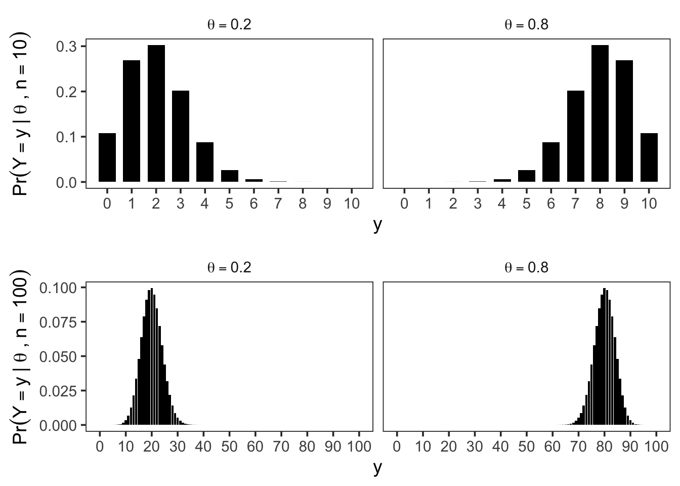
In the case where \(Y_1, \ldots, Y_n \mid \theta\) are i.i.d. Bernoulli\((\theta)\) random variables, the sufficient statistic \(Y = \sum_{i=1}^n Y_i\) follows a binomial distribution with parameters \((n, \theta)\).

The Binomial Model

Because each \(Y_i\) is Bernoulli\((\theta)\) and the observations are independent, the sufficient statistic \(Y = \sum_{i=1}^n Y_i\) follows a binomial distribution with parameters \((n, \theta)\).

That is, \(\Pr(Y = y \mid \theta)=\binom{n}{y} \theta^y (1 - \theta)^{n - y}\), \(y = 0, 1, \ldots, n\). For a binomial\((n, \theta)\) random variable \(Y\),

\(\mathbb{E}[Y \mid \theta] = n\theta\),
\(\mathrm{Var}(Y \mid \theta) = n\theta(1 - \theta).\)

Posterior inference under a uniform prior distribution

Having observed \(Y = y\) our task is to obtain the posterior distribution of \(\theta\). By Bayes’ theorem, \[ p(\theta \mid y) = \frac{p(y \mid \theta),\pi(\theta)}{p(y)}. \]

For a binomial model with \(Y \sim \text{Binomial}(n,\theta)\), the likelihood is \[ p(y \mid \theta) = \binom{n}{y}\theta^y(1-\theta)^{n-y}. \]

Therefore, \[ p(\theta \mid y) = \frac{\binom{n}{y} \theta^y(1-\theta)^{n-y}\pi(\theta)}{p(y)} = c(y) \theta^y(1-\theta)^{n-y}\pi(\theta), \] where \(c(y)\) is a normalizing constant that depends only on \(y\), not on \(\theta\). When using the uniform distribution, \(\pi(\theta)\), we can calculate \(c(y)\) easily as \[ \begin{aligned} 1&=\int_0^1 c(y) \theta^y(1-\theta)^{n-y} d \theta \\ &=c(y) \int_0^1 \theta^y(1-\theta)^{n-y} d \theta \\ &=c(y) \frac{\Gamma(y+1) \Gamma(n-y+1)}{\Gamma(n+2)} \end{aligned}. \] Hence, \(c(y)=\Gamma(n+2)/\{\Gamma(y+1) \Gamma(n-y+1)\}\), and the posterior distribution is \[ \begin{aligned} p(\theta \mid y) & =\frac{\Gamma(n+2)}{\Gamma(y+1) \Gamma(n-y+1)} \theta^y(1-\theta)^{n-y} \\ & =\frac{\Gamma(n+2)}{\Gamma(y+1) \Gamma(n-y+1)} \theta^{(y+1)-1}(1-\theta)^{(n-y+1)-1}, \end{aligned} \] Which is exactly the \(\operatorname{beta}(y+1, n-y+1)\). In the happiness example, we have \(n=129\) and \(Y=\sum Y_i=118\), so the posterior distribution is \(\operatorname{beta}(119,12)\), written as \[ n=129, Y \equiv \sum Y_i=118 \quad \Rightarrow \quad \theta \mid\{Y=118\} \sim \operatorname{beta}(119,12) . \]

This confirms the sufficiency result for this model and prior distribution, by showing that if \(\sum y_i = y = 118\), \(p(\theta\mid y_1,\dots y_n) = p(\theta\mid y) = \mathrm{beta}(119, 12)\). That is, the information contained in \(\{Y_1 = y_1, \dots, Y_n = y_n\}\) is the same as the information contained in \(\{Y = y\}\), where \(Y = \sum Y_i\) and \(y = \sum y_i\). This show the posterior when we use uniform prior. One may ask, what if we use a different prior?

Posterior distributions under beta prior distributions

The uniform prior distribution has \(\pi(\theta) = 1\) for all \(\theta\in [0,1]\). This distribution can be thought of as a beta prior distribution with parameters \(a = 1, b = 1\) \[ \pi(\theta)=\frac{\Gamma(2)}{\Gamma(1) \Gamma(1)} \theta^{1-1}(1-\theta)^{1-1}=\frac{1}{1 \times 1} 1 \times 1=1 \] for all \(\theta \in[0,1]\).

The gamma function is defined as \[ \Gamma(x)=\int_0^{\infty} t^{x-1} e^{-t} d t, \quad x>0. \]

It satisfies the following properties:

\(\Gamma(n)=(n-1)!\) for any positive integer \(n\).
\(\Gamma(x+1)=x \Gamma(x)\) for any \(x>0\).
\(\Gamma(1 / 2)=\sqrt{\pi}\).
\(\Gamma(1)=1\) by convention.

Now, from the previous part, recall that we have, \[ \text { if }\left\{\begin{array}{c} \theta \sim \operatorname{beta}(1,1) \text { (uniform) } \\ Y \sim \operatorname{binomial}(n, \theta) \end{array}\right\}, \text { then }\{\theta \mid Y=y\} \sim \operatorname{beta}(1+y, 1+n-y). \]

To get the posterior distribution under a general beta prior distribution, we just need to add the number of 1’s to the \(\alpha\) parameter and the number of 0’s to the \(\beta\) parameter. To see this, assume \(\theta\sim \operatorname{beta}(\alpha, \beta)\), and \(Y\mid \theta \sim \operatorname{binomial}(n, \theta)\). Then, once we observed \(\{Y=y\}\), by Bayes’ theorem, the posterior distribution is \[ \begin{aligned} p(\theta \mid y) & =\frac{\pi(\theta) p(y \mid \theta)}{p(y)} \\ & =\frac{1}{p(y)} \times \frac{\Gamma(a+b)}{\Gamma(a) \Gamma(b)} \theta^{a-1}(1-\theta)^{b-1} \times\binom{ n}{y} \theta^y(1-\theta)^{n-y} \\ & =c(n, y, a, b) \times \theta^{a+y-1}(1-\theta)^{b+n-y-1} \\ &\propto \beta(a+y, b+n-y) . \end{aligned} \]

One-to-one correspondence between the distribution

Note that, there is a one-to-one correspondence between the prior distribution parameters and the posterior distribution parameters. Two distributions are said to be the same if

Their CDFs are the same.
Their PDFs are the same.
All of their moments are the same. This implies that they are equal if and only if the moment generating function or the probability generating functions are the same.

We have seen the beta-binomial example twice, which is an example of conjugate prior, let’s definite this formally,

A class \(\mathcal{P}\) of prior distribution for \(\theta\) is said conjugate for the likelihood function \(p(y \mid \theta)\) if for every prior distribution \(\pi(\theta) \in \mathcal{P}\), the corresponding posterior distribution \(p(\theta \mid y)\) is also in \(\mathcal{P}\), that is \[ \pi(\theta) \in \mathcal{P} \Rightarrow p(\theta \mid y) \in \mathcal{P}. \]

Note

Conjugate priors simplify posterior calculations, but they may not accurately reflect genuine prior beliefs. Still, mixtures of conjugate priors offer substantially greater flexibility while remaining computationally tractable.

If the likelihood \(\theta \mid \{Y = y\} \sim beta(a + y, b + n − y)\), recall that

\(\mathrm{E}[\theta \mid y]=\frac{a+y}{a+b+n}\)
\(\operatorname{mode}[\theta \mid y]=\frac{a+y-1}{a+b+n-2}\)
\(\operatorname{Var}[\theta \mid y]=\frac{\mathrm{E}[\theta \mid y] \mathrm{E}[1-\theta \mid y]}{a+b+n+1}\)

The posterior mean can be expressed as a weighted average of the prior mean and the maximum likelihood estimate (MLE) of \(\theta\): \[ \begin{aligned} \mathrm{E}[\theta \mid y] & =\frac{a+y}{a+b+n} \\ & =\frac{a+b}{a+b+n} \times\frac{a}{a+b}+\frac{n}{a+b+n}\times \frac{y}{n} \\ & =\frac{a+b}{a+b+n} \times \text { prior expectation }+\frac{n}{a+b+n} \times \text { data mean } \end{aligned} \] For this model and prior distribution, the posterior expectation (also known as the posterior mean) can be expressed as a weighted average of the prior expectation and the sample mean. The weights are proportional to the prior sample size a + b and the observed sample size n, respectively. This representation leads to a natural interpretation of the Beta prior parameters as prior data:

\(a \approx \text{``prior \# of 1’s,''}\)
\(b \approx \text{``prior \# of 0’s,''}\)
\(a + b \approx \text{``prior sample size.''}\)

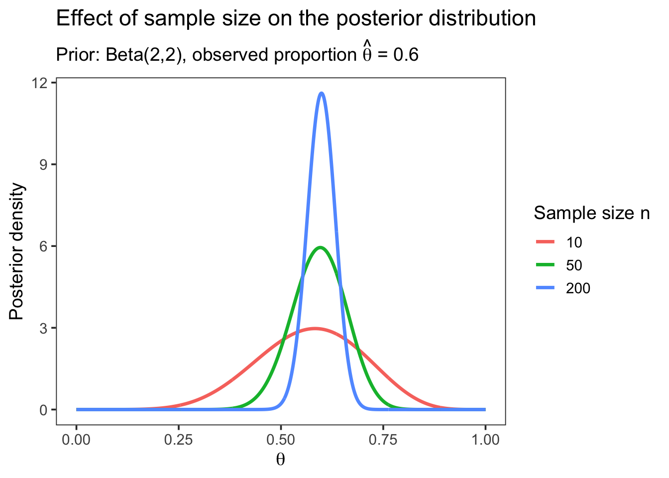
When \(n \gg a+b\), it is reasonable to expect that most of the information about \(\theta\) should come from the data rather than from the prior distribution. This intuition is confirmed mathematically. In particular, when \(n \gg a + b\),

\(\frac{a + b}{a + b + n} \approx 0\),
\(\mathbb{E}[\theta \mid y] \approx \frac{y}{n}\),
\(\mathrm{Var}(\theta \mid y) \approx \frac{1}{n}\,\frac{y}{n}\left(1 - \frac{y}{n}\right)\).

Thus, in large samples, the posterior mean approaches the sample proportion and the posterior variance shrinks at rate \(1/n\), reflecting increasing information from the data.

Prediction

An important feature of Bayesian inference is the existence of a predictive distribution for new observations.

The posterior predictive distribution for a new observation \(Y_{\text{new}}\) given the observed data \(y\) is obtained by integrating over the posterior distribution of \(\theta\).

Returning to our notation for binary data, let \(y_1, \ldots, y_n\) be the observed outcomes from a sample of \(n\) binary rvs, and let \(\tilde Y \in \{0,1\}\) denote a future observation from the same population that has not yet been observed. The predictive distribution of \(\tilde Y\) is defined as the conditional distribution of \(\tilde Y\) given the observed data \(\{Y_1=y_1,\ldots,Y_n=y_n\}\). For conditionally i.i.d. binary observations, the predictive distribution can be derived by integrating out the unknown parameter \(\theta\): \[ \begin{aligned} \operatorname{Pr}\left(\tilde{Y}=1 \mid y_1, \ldots, y_n\right) & =\int \operatorname{Pr}\left(\tilde{Y}=1, \theta \mid y_1, \ldots, y_n\right) d \theta \\ & =\int \operatorname{Pr}\left(\tilde{Y}=1 \mid \theta, y_1, \ldots, y_n\right) p\left(\theta \mid y_1, \ldots, y_n\right) d \theta \\ & =\int p\left(\theta \mid y_1, \ldots, y_n\right) \theta d \theta \\ & =\mathrm{E}\left[\theta \mid y_1, \ldots, y_n\right]\\ &=\frac{a+\sum_{i=1}^n y_i}{a+b+n}. \end{aligned} \]

Hence, we also have, \[ \operatorname{Pr}\left(\tilde{Y}=0 \mid y_1, \ldots, y_n\right) =1-\mathrm{E}\left[\theta \mid y_1, \ldots, y_n\right]=\frac{b+\sum_{i=1}^n\left(1-y_i\right)}{a+b+n} . \]

Properties of the predictive distribution

It does not depend on any unknown quantities. If it did, it could not be used to make predictions.
It depends on the observed data. In particular, \(\tilde Y\) is not independent of \(Y_1,\ldots,Y_n\), because the observed data provide information about \(\theta\), which in turn influences \(\tilde Y\). If \(\tilde Y\) were independent of the observed data, learning from data would be impossible.

The uniform prior distribution on [0,1], also known as the \(\text{Beta}(1,1)\) prior, can be interpreted as containing the same information as a hypothetical prior dataset consisting of one success (“1”) and one failure (“0”).

Under this prior, the posterior predictive probability of a future success is \[ \Pr(\tilde Y = 1 \mid Y = y) = \mathbb{E}[\theta \mid Y = y] = \frac{2}{2+n}\cdot\frac{1}{2} + \frac{n}{2+n}\cdot\frac{y}{n}. \]

This expression highlights that the predictive probability is a weighted average of:

the prior mean \(1/2\), and
the sample proportion \(y/n\),

with weights proportional to the prior sample size 2 and the observed sample size n, respectively.

The posterior mode under this prior is \[ \text{mode}(\theta \mid Y = y) = \frac{y}{n}, \] where \[ Y = \sum_{i=1}^n Y_i. \]

At first glance, the discrepancy between these two posterior summaries may seem surprising. However, it reflects the fact that different summaries capture different features of the posterior distribution.

To see this clearly, consider the case \(Y = 0\). In this case, \[ \text{mode}(\theta \mid Y = 0) = 0, \] but the predictive probability remains \[ \Pr(\tilde Y = 1 \mid Y = 0) = \frac{1}{2+n}. \]

Thus, even when no successes have been observed, the Bayesian predictive distribution assigns a positive probability to a future success due to the prior information. This illustrates how Bayesian prediction naturally balances prior beliefs with observed data.

3.2.2 Confidence Regions: Bayesian v.s. Frequentist

If it often desirable to identify the regions of the parameter space that are likely to contain the true value of the parameter. To do this, after observing the data \(Y=y\), we can construct an interval \([\ell(y),u(y)]\) that is likely to contain the true value of \(\theta\), i.e., the probability that \(\ell(y)<\theta<u(y)\) is large. There are two different ways to interpret this probability, leading to the concepts of Bayesian coverage and frequentist coverage.

An interval \([\ell(y), u(y)]\), based on the observed data \(Y = y\), has 100(1-\(\alpha\))% Bayesian coverage for \(\theta\) if \[ \Pr(\ell(y) < \theta < u(y)\mid Y = y) = 1-\alpha. \]

A random interval \([\ell(Y ), u(Y )]\) has 100(1-\(\alpha\))% frequentist coverage for \(\theta\) if, before the data are gathered, \[ \Pr(\ell(Y ) < \theta < u(Y )\mid\theta) = 1-\alpha. \]

Note

In a sense, the frequentist and Bayesian notions of coverage describe pre experimental and post experimental perspectives, respectively.

3.3 Frequentist vs Bayesian Coverage

You may recall an important point often emphasized in introductory statistics courses. Suppose we observe data \(Y=y\) and compute a frequentist confidence interval \[ [l(y),\,u(y)]. \] Once the data are observed, the parameter \(\theta\) is treated as fixed, not random.
Therefore, \[ \Pr\!\bigl(l(y) < \theta < u(y) \mid \theta\bigr) = \begin{cases} 1, & \text{if } \theta \in [l(y),u(y)],\\ 0, & \text{if } \theta \notin [l(y),u(y)]. \end{cases} \]

This highlights a key limitation of frequentist confidence intervals:

They do not admit a post-experimental probability interpretation.

After observing the data, it is not meaningful, from a frequentist perspective, to say that there is a 95% probability that \(\theta\) lies in the computed interval.

What Frequentist Coverage Means

Although this interpretation may feel unsatisfying, frequentist coverage is still useful in many situations. Imagine repeatedly running many independent experiments and constructing a confidence interval for each one.
If each interval procedure has 95% frequentist coverage, then:

About 95% of the intervals will contain the true parameter value.

This is a long-run, repeated-sampling interpretation, not a statement about any single observed interval.

Can Bayesian and Frequentist Coverage Agree?

A natural question is whether a confidence interval can simultaneously have:

a Bayesian interpretation, i.e., a 100(1-\(\alpha\))% posterior probability that \(\theta\) lies in the interval, and
approximately 100(1-\(\alpha\))% frequentist coverage.

Hartigan (1966) showed that, for the types of intervals considered in Hopf (2009), an interval that has 95% Bayesian coverage additionally has the property that \[ \Pr\!\bigl(l(Y) < \theta < u(Y) \mid \theta\bigr) = 0.95 + \varepsilon_n, \] where the error term satisfies \(|\varepsilon_n| < a/n\) for some constant \(a\). This result implies that, an interval with 95% Bayesian coverage, will also have approximately 95% frequentist coverage, at least asymptotically, as the sample size \(n\) grows.

In other words, under suitable conditions, Bayesian credible intervals and frequentist confidence intervals can agree in large samples, even though their interpretations are fundamentally different. Keep in mind that most non-Bayesian methods of constructing 100(1-\(\alpha\))% confidence intervals also only achieve their nominal coverage probability asymptotically.

Reminder

This reconciliation is important, but it should not obscure the conceptual distinction:

frequentist coverage is a pre-experimental property of a procedure,
Bayesian coverage is a post-experimental probability statement about \(\theta\) given the data.

For further discussion of the similarities between Bayesian and frequentist intervals, see Severini (1991) and Sweeting (2001).

3.4 Posterior Quantile Intervals

One of the simplest ways to construct a Bayesian credible interval is to use posterior quantiles. To form a \(100(1-\alpha)\%\) credible interval for \(\theta\), find numbers \(\theta_{\alpha/2} < \theta_{1-\alpha/2}\) such that

\(\Pr(\theta < \theta_{\alpha/2} \mid Y=y) = \alpha/2,\)
\(\Pr(\theta > \theta_{1-\alpha/2} \mid Y=y) = \alpha/2,\)

where \(\theta_{\alpha/2}\) and \(\theta_{1-\alpha/2}\) are the \(\alpha/2\) and \(1-\alpha/2\) posterior quantiles of \(\theta\). By construction, \[ \begin{aligned} \operatorname{Pr}\left(\theta \in\left[\theta_{\alpha / 2}, \theta_{1-\alpha / 2}\right] \mid Y=y\right) & =1-\operatorname{Pr}\left(\theta \notin\left[\theta_{\alpha / 2}, \theta_{1-\alpha / 2}\right] \mid Y=y\right) \\ & =1-\left[\operatorname{Pr}\left(\theta<\theta_{\alpha / 2} \mid Y=y\right)+\operatorname{Pr}\left(\theta>\theta_{1-\alpha / 2} \mid Y=y\right)\right] \\ & =1-\alpha . \end{aligned} \]

Suppose we observe \(n = 10\) conditionally independent Bernoulli trials and obtain \(Y = 2\) successes. Using a uniform prior for \(\theta\), \(\theta \sim \mathrm{Beta}(1,1),\) the posterior distribution is \[ \theta \mid \{Y=2\} \sim \mathrm{Beta}(1+2,\;1+8) = \mathrm{Beta}(3,9). \]

A 95% posterior confidence interval can be obtained from by 2.5% and 97.5% quantiles of this Beta distribution \([\theta_{0.025}, \theta_{0.975}]\). In this case, \[ \theta_{0.025} \approx 0.06, \qquad \theta_{0.975} \approx 0.52, \] so \[ \Pr(0.06 \le \theta \le 0.52 \mid Y=2) = 0.95. \]

This interval has a direct probabilistic interpretation: given the observed data, there is a 95% posterior probability that \(\theta\) lies in this range.

b <- a <- 1 # prior parameter
n <- 10 ; y <- 2 # data
qbeta(c(0.025, 0.975), a + y, b + n - y)

[1] 0.06021773 0.51775585

a_post <- a + y
b_post <- b + (n - y)

# 95% quantile-based credible interval
ci <- qbeta(c(0.025, 0.975), a_post, b_post)
ci_low <- ci[1]
ci_high <- ci[2]

# Grid for plotting posterior density
theta <- seq(0, 1, length.out = 2000)
df <- data.frame(theta = theta, density = dbeta(theta, a_post, b_post))

# Plot: posterior density curve + two vertical CI bars
ggplot(df, aes(x = theta, y = density)) +
  geom_line(linewidth = 1) +
  geom_vline(xintercept = ci_low, linewidth = 0.8) +
  geom_vline(xintercept = ci_high, linewidth = 0.8) +
  labs(
    title = "Beta Posterior with 95% Quantile-Based Credible Interval",
    subtitle = sprintf(
      "Data: n=%d, y=%d | Prior: Beta(%d,%d) | Posterior: Beta(%d,%d) | 95%% CI: [%.3f, %.3f]",
      n, y, a, b, a_post, b_post, ci_low, ci_high
    ),
    x = expression(theta),
    y = expression(p(theta * "|" * y))
  ) +
  theme_minimal()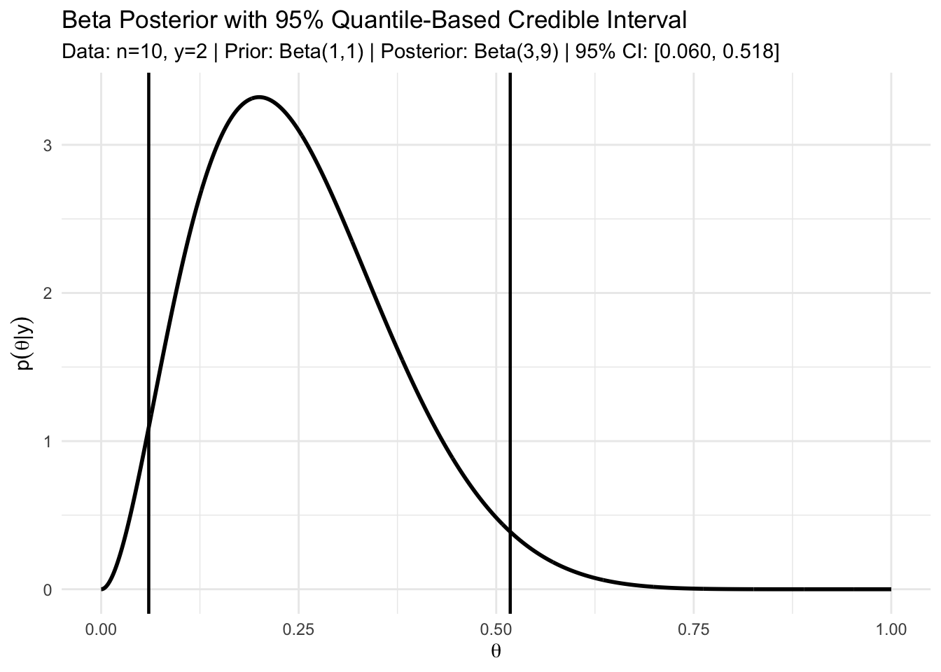

Highest posterior density (HPD) region

The Figure above illustrates the posterior distribution of \(\theta\) for the binomial example with a uniform prior, together with a 95% quantile-based credible interval. Notice an important feature of the plot:

There exist values of \(\theta\) outside the quantile-based interval that have higher posterior density than some values inside the interval.

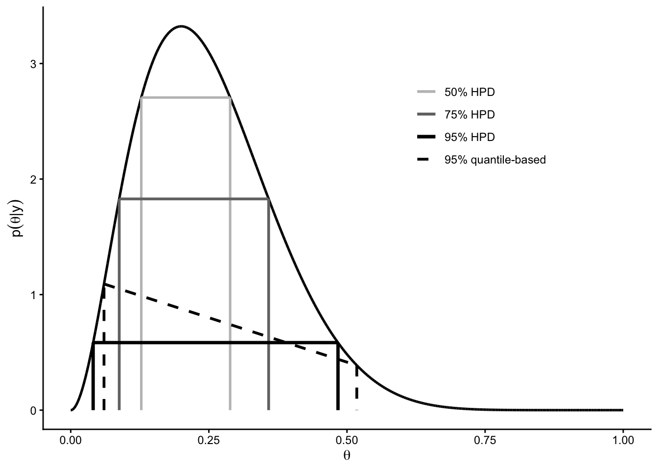
This observation suggests that the quantile-based interval may not be the most efficient way to summarize posterior uncertainty. In particular, it motivates a more restrictive type of credible region that concentrates on the most plausible parameter values.

A \(100(1-\alpha)\%\) HPD region is a subset of the sample space, \(s(y) \subset \Theta\) such that:

\(\Pr(\theta \in s(y) \mid Y = y) = 1 - \alpha\), and
If \(\theta_a \in s(y)\) and \(\theta_b \notin s(y)\), then \(p(\theta_a \mid Y = y) \ge p(\theta_b \mid Y = y).\)

In words, an HPD region contains the parameter values with the largest posterior density, subject to containing probability mass \(1-\alpha\).

Observed that, all points inside an HPD region are at least as plausible as any point outside the region, according to the posterior distribution. This property distinguishes HPD regions from quantile-based intervals, which are defined purely by cumulative probability and may include low-density values while excluding higher-density ones.

An HPD region can be constructed conceptually as follows:

Algorithm to construct an HPD region

Begin with a horizontal line above the posterior density curve.
Gradually lower the line.
At each height, include all values of \(\theta\) whose posterior density exceeds the line.
Stop lowering the line once the total posterior probability of the included region reaches \(1-\alpha\).

This procedure guarantees that the retained region consists of the most probable values of \(\theta\).

HPD Regions and Multimodality

If the posterior density is unimodal, the HPD region will typically be a single interval. However, if the posterior density is multimodal (having multiple peaks), the HPD region need not be an interval; it may consist of several disjoint subsets of the parameter space.

In the binomial example with \(n=10\), \(Y=2\), and a uniform prior, the posterior distribution is \(\mathrm{Beta}(3,9)\).

For this posterior:

The 95% quantile-based credible interval is approximately \([0.06,\,0.52]\).
The 95% HPD region is approximately \([0.04,\,0.48]\).

The HPD region is narrower, and therefore more precise, than the quantile-based interval, while still containing 95% of the posterior probability.

Both intervals are valid Bayesian credible intervals, but they summarize posterior uncertainty in different ways.

3.5 The Poisson Model

Another commonly used distribution is the Poisson, in this case, the measurement are the integer numbers. Some examples include number of coin tosses, the number of friends they have, or the number of birthday celebrations have a person have. In these situations, the sample space is \(\mathcal{Y}=\{0,1,2,\ldots\}.\) There are other possible models for those situation, but perhaps the simplest probability model on \(\mathcal{Y}\) is the Poisson model.

Poisson distribution

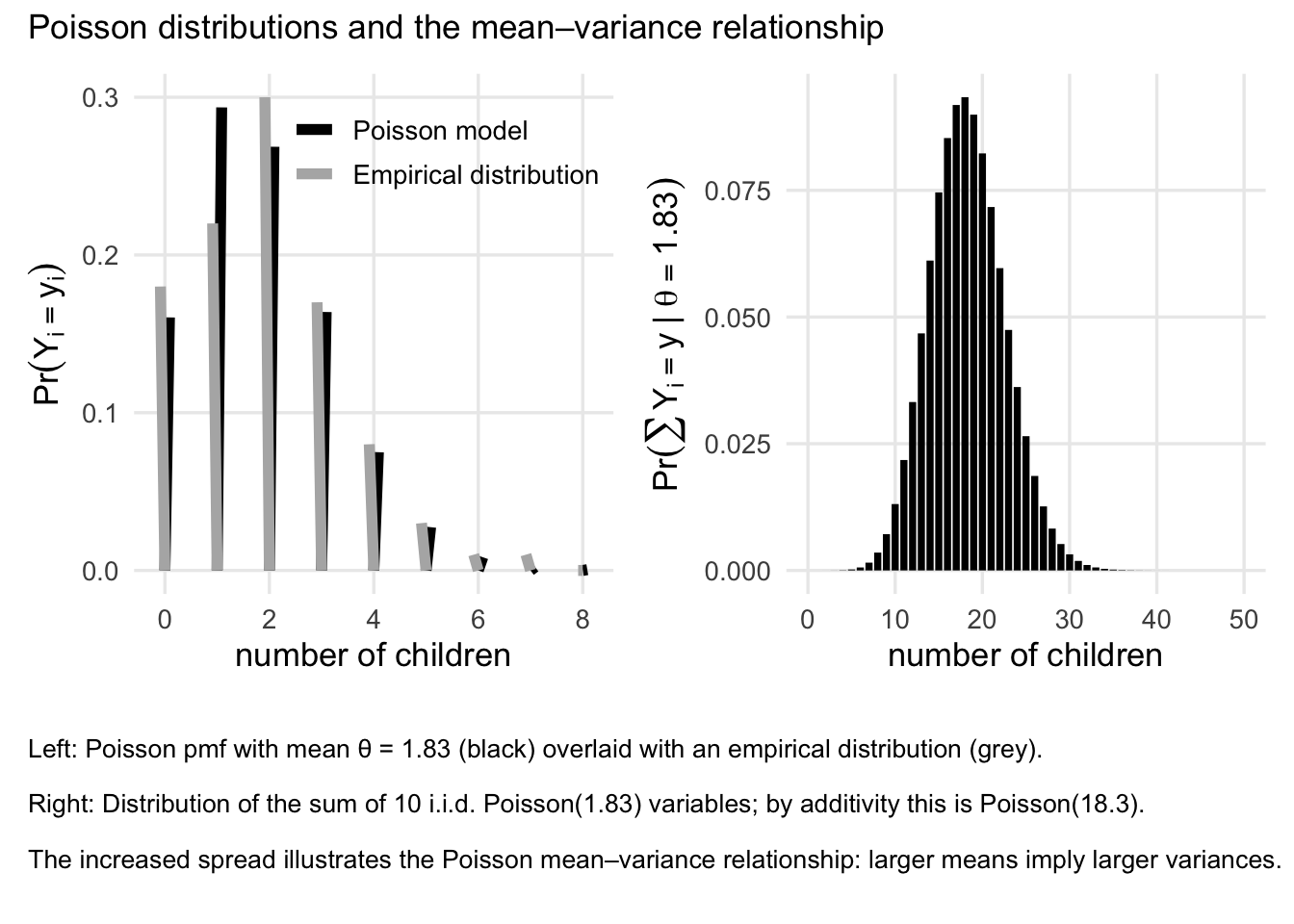
Recall that a random variable \(Y\) has a Poisson distribution with mean \(\theta\) if \[ \Pr(Y=y\mid \theta)=\mathrm{dpois}(y,\theta)=\frac{\theta^y e^{-\theta}}{y!}, \qquad y\in\{0,1,2,\ldots\}. \]

For such a random variable, we have,

\(\mathbb{E}(Y)=\theta\)
\(\mathrm{Var}(Y)=\theta.\)

People sometimes use the Poisson distribution to model count data because of its simplicity and its ability to model events that occur independently over a fixed interval of time or space. The Poisson distribution is particularly useful when the events being counted are rare or infrequent, and when the average rate of occurrence is known. Note that, in this model, the mean and the variance are the same, which is a property that can be useful in certain applications; One may call this property as “mean-variance relationship”.

3.5.1 Inference on the Posterior for Poisson Model

Suppose we observe data \(Y_1, \ldots, Y_n\) and model them as conditionally independent Poisson random variables with common mean \(\theta\), i.e., \[ Y_i \mid \theta \sim \text{Poisson}(\theta), \qquad i = 1,\ldots,n. \]

The joint probability mass function of the data, given \(\theta\), is \[ \Pr(Y_1 = y_1, \ldots, Y_n = y_n \mid \theta) = \prod_{i=1}^n p(y_i \mid \theta). \]

Using the Poisson pmf, \[ p(y_i \mid \theta) = \frac{\theta^{y_i} e^{-\theta}}{y_i!}, \] we obtain \[ \begin{aligned} \Pr(Y_1 = y_1, \ldots, Y_n = y_n \mid \theta) &= \prod_{i=1}^n \frac{\theta^{y_i} e^{-\theta}}{y_i!}\\ &= c(y_1,\ldots,y_n)\,\theta^{\sum_{i=1}^n y_i} e^{-n\theta}, \end{aligned} \] where \[ c(y_1,\ldots,y_n) = \prod_{i=1}^n \frac{1}{y_i!}, \] which does not depend on \(\theta\). This expression shows that the likelihood depends on the data only through the statistic \(S = \sum_{i=1}^n Y_i.\)

As in the binomial model, the statistic \(S = \sum_{i=1}^n Y_i\) contains all information in the data about \(\theta\).
Indeed, \[ \sum_{i=1}^n Y_i \mid \theta \sim \text{Poisson}(n\theta), \] and we therefore say that \(S\) is a sufficient statistic for \(\theta\).

3.5.2 Comparing posterior beliefs

To compare two values \(\theta_a\) and \(\theta_b\) a posteriori, consider the posterior odds: \[ \frac{p(\theta_a \mid y_1,\ldots,y_n)} {p(\theta_b \mid y_1,\ldots,y_n)}. \]

By Bayes’ rule, \[ p(\theta \mid y_1,\ldots,y_n) \propto \pi(\theta)\,p(y_1,\ldots,y_n \mid \theta) \propto \pi(\theta)\,\theta^{\sum_{i=1}^n y_i} e^{-n\theta}. \]

Therefore, \[ \frac{p(\theta_a \mid y)} {p(\theta_b \mid y)} = \frac{\theta_a^{\sum y_i} e^{-n\theta_a} p(\theta_a)} {\theta_b^{\sum y_i} e^{-n\theta_b} p(\theta_b)}. \]

This expression highlights how posterior beliefs balance prior information with evidence from the data.

Conjugate prior for the Poisson model

We now seek a prior distribution for \(\theta\) that leads to a posterior distribution of the same functional form. From the likelihood, \[ p(\theta \mid y) \propto p(\theta)\,\theta^{\sum y_i} e^{-n\theta}, \] we see that a conjugate prior must involve terms of the form \[ \theta^{c_1} e^{-c_2 \theta} \] for some constants \(c_1\) and \(c_2\). The simplest family of distributions with this structure is the family of Gamma distributions, also called Gamma family.

3.5.3 Gamma distribution

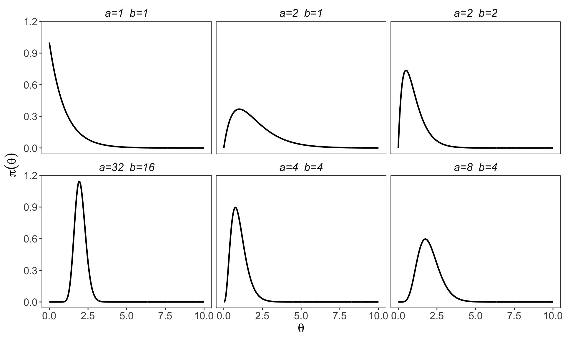
A positive random variable \(\theta\) has a Gamma\((a,b)\) distribution if \[ \pi(\theta) = \frac{b^a}{\Gamma(a)} \theta^{a-1} e^{-b\theta}, \qquad \theta > 0, \] where \(a > 0\) is the shape parameter and \(b > 0\) is the rate parameter.

For a Gamma\((a,b)\) random variable,

\(\mathbb{E}(\theta) = a/b,\)
\(\mathrm{Var}(\theta) = a/b^2.\)
\(\operatorname{mode}[\theta]=\left\{\begin{array}{cc} (a-1) / b & \text { if } a>1 \\ 0 & \text { if } a \leq 1 \end{array} .\right.\)

3.5.4 Posterior distribution of \(\theta\)

If the prior is \(\theta \sim \text{Gamma}(a,b),\) then combining the prior with the Poisson likelihood yields \[ \begin{aligned} p\left(\theta \mid y_1, \ldots, y_n\right) & =\pi(\theta) \times p\left(y_1, \ldots, y_n \mid \theta\right) / p\left(y_1, \ldots, y_n\right) \\ & =\left\{\theta^{a-1} e^{-b \theta}\right\} \times\left\{\theta^{\sum y_i} e^{-n \theta}\right\} \times c\left(y_1, \ldots, y_n, a, b\right) \\ & =\left\{\theta^{a+\sum y_i-1} e^{-(b+n) \theta}\right\} \times c\left(y_1, \ldots, y_n, a, b\right)\\ &\propto \theta^{a+\sum y_i-1} e^{-(b+n)\theta}. \end{aligned} \]

Thus, by the uniqueness theorem (of the density), the posterior distribution is \[ \theta \mid y_1,\ldots,y_n \sim \text{Gamma}\big(a + \sum_{i=1}^n y_i,\; b + n\big). \]

This shows that the Gamma distribution is conjugate to the Poisson likelihood.

Interpretation

Posterior inference for the Poisson model is therefore straightforward:

The data enter only through the sufficient statistic \(\sum Y_i\);
The posterior mean is \[ \begin{aligned} \mathrm{E}\left[\theta \mid y_1, \ldots, y_n\right] & =\frac{a+\sum y_i}{b+n} \\ & =\frac{b}{b+n} \frac{a}{b}+\frac{n}{b+n} \frac{\sum y_i}{n} \end{aligned} \]
This decomposition shows that it is a convex combination of the prior mean \(a/b\) and the sample mean \(\bar{y}\), and gives a useful information
\(b\) acts like the number of prior observations;
\(a\) acts like the total count from those \(b\) observations;
\(a/b\) is the prior mean.
Increasing the sample size \(n\) reduces posterior uncertainty, because the ifnromation from the data dominates the prior belief. To see this, we have, for \(n\gg b\), we have
\(\mathrm{E}[\theta \mid y] \approx \bar{y}\),
\(\mathrm{Var}(\theta \mid y) \approx \bar{y}/n\).

This conjugate structure makes the Poisson–Gamma model a convenient and interpretable starting point for Bayesian analysis of count data.

3.5.5 Posterior predictive distribution for Poisson Model

We have seen that, the Bayesian prediction for a future observation \(\tilde{y}\) is based on the posterior predictive distribution. In Gamma-Poisson model, we have \[ p(\tilde{y} \mid y_1,\ldots,y_n) = \int_0^\infty p(\tilde{y} \mid \theta, y)\, p(\theta \mid y_1,\ldots,y_n) \, d\theta. \]

For the Poisson model, \[ p(\tilde{y} \mid \theta) = \text{Poisson}(\theta), \qquad p(\theta \mid y) = \text{Gamma}\!\left(a + \sum y_i,\; b + n\right). \]

Substituting, \[ p(\tilde{y} \mid y) = \int_0^\infty \text{dpois}(\tilde{y},\theta)\, \text{dgamma}\!\left(\theta,\; a + \sum y_i,\; b + n\right) \, d\theta. \]

Writing this integral explicitly, \[ p(\tilde{y} \mid y) = \int_0^\infty \frac{\theta^{\tilde{y}} e^{-\theta}}{\tilde{y}!} \cdot \frac{(b+n)^{a+\sum y_i}}{\Gamma(a+\sum y_i)} \theta^{a+\sum y_i-1} e^{-(b+n)\theta} \, d\theta. \]

Combining terms, we have \[ p(\tilde{y} \mid y) = \frac{(b+n)^{a+\sum y_i}}{\tilde{y}!\,\Gamma(a+\sum y_i)} \int_0^\infty \theta^{a+\sum y_i+\tilde{y}-1} e^{-(b+n+1)\theta} \, d\theta. \]

The integral term seems difficult to evaluate in a glance, but there is actually a clear “trick” to help use. Recall the density of a Gamma distribution: \[ 1 = \int_0^\infty \frac{\beta^\alpha}{\Gamma(\alpha)} \theta^{\alpha-1} e^{-\beta\theta}\, d\theta, \quad, \alpha,\beta>0, \] which implies \[ \int_0^\infty \theta^{\alpha-1} e^{-\beta\theta}\, d\theta = \frac{\Gamma(\alpha)}{\beta^\alpha}, \qquad \alpha,\beta>0. \]

Applying this with \[ \alpha = a + \sum y_i + \tilde{y}, \qquad \beta = b + n + 1, \] we obtain \[ \int_0^\infty \theta^{a+\sum y_i+\tilde{y}-1} e^{-(b+n+1)\theta} \, d\theta = \frac{\Gamma(a+\sum y_i+\tilde{y})}{(b+n+1)^{a+\sum y_i+\tilde{y}}}. \]

Substituting back and simplifying, \[ p(\tilde{y} \mid y_1,\ldots,y_n) = \frac{\Gamma(a+\sum y_i+\tilde{y})}{\Gamma(a+\sum y_i)\,\tilde{y}!} \left(\frac{b+n}{b+n+1}\right)^{a+\sum y_i} \left(\frac{1}{b+n+1}\right)^{\tilde{y}}, \] for \(\tilde{y} \in \{0,1,2,\ldots\}\). We relieazed that it is a negative binomial distribution with parameters \((a + \sum y_i, b + n)\). That is, \(\tilde{Y} \mid y_1,\ldots,y_n \sim \text{NB}(a + \sum y_i, b + n)\). As a result, we have the mean and variance of the posterior predictive distribution

\[\mathbb{E}(\tilde{Y} \mid y) = \frac{a + \sum y_i}{b + n}=\mathbb{E}[\theta \mid y], \]

and

\[ \begin{aligned} \mathrm{Var}\left[\tilde{Y} \mid y_1, \ldots, y_n\right] & =\frac{a+\sum y_i}{b+n} \frac{b+n+1}{b+n}\\ &=\operatorname{Var}\left[\theta \mid y_1, \ldots y_n\right] \times(b+n+1) \\ & =\mathbb{E}\left[\theta \mid y_1, \ldots, y_n\right] \times \frac{b+n+1}{b+n} \\ & = \frac{a + \sum y_i}{b + n} \times \frac{b + n + 1}{b + n} \end{aligned}, \] respectively

Interpretation and Take away

Recall that the predictive variance is to some extent a measure of our posterior uncertainty about a new observation \(\tilde{Y}\). It reflects two sources of uncertainty:

Sampling variability (Sampling) For a Poisson model, the variance of \(Y\) given \(\theta\) is equal to \(\theta\).
Parameter uncertainty (Population) When \(\theta\) is unknown, uncertainty about \(\theta\) inflates the variance of future observations.

For large \(n\), the data dominate the prior: \[ \frac{b + n + 1}{b + n} \approx 1, \] so predictive uncertainty is driven primarily by sampling variability. In this case, the uncertainy abbout \(\theta\) is small which for the Possion model is equal to \(theta\)

For small \(n\), posterior uncertainty about \(\theta\) is substantial, and \[ \frac{b + n + 1}{b + n} > 1, \] leading to larger predictive variance than under a fixed-\(\theta\) Poisson model (i.e., larger than just the sampling variability).

Bayesian prediction naturally incorporates both sampling variability and parameter uncertainty.

This completes posterior inference and prediction for the Gamma-Poisson model.

3.6 Example: Birth rates

Over the course of the 1990s, the General Social Survey collected data on the educational attainment and number of children of women who were 40 years old at the time of participation in the survey. These women were in their 20s during the 1970s, a period of historically low fertility rates in the United States.

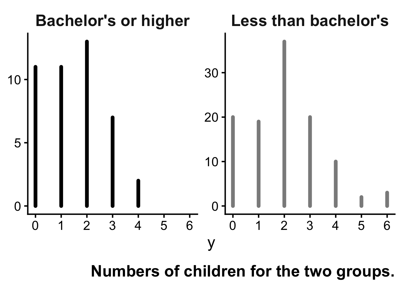
In this example, we compare women with a bachelor’s degree to those without a bachelor’s degree in terms of their numbers of children.

Sampling models

Let

\(Y_{i,1}\) denote the number of children for woman \(i\) without a bachelor’s degree, \(i=1,\dots,n_1\),
\(Y_{i,2}\) denote the number of children for woman \(i\) with a bachelor’s degree, \(i=1,\dots,n_2\).

Then, since it is a coint data, we assume the following Poisson sampling models:

\[ Y_{1,1}, \ldots, Y_{n_1,1} \mid \theta_1 \sim \text{i.i.d. Poisson}(\theta_1), \]

\[ Y_{1,2}, \ldots, Y_{n_2,2} \mid \theta_2 \sim \text{i.i.d. Poisson}(\theta_2). \]

Here, \(\theta_1\) and \(\theta_2\) represent the population mean birth rates for the two groups.

Data summaries

The empirical summaries of the data are:

No college degree: \[ n_1 = 111, \qquad \sum_{i=1}^{n_1} Y_{i,1} = 217, \qquad \bar{Y}_1 = 1.95 \]
Bachelor’s degree or higher: \[ n_2 = 44, \qquad \sum_{i=1}^{n_2} Y_{i,2} = 66, \qquad \bar{Y}_2 = 1.50 \]

Prior distributions

We place independent Gamma priors on the two population means:

\[ \theta_1, \theta_2 \sim \text{i.i.d. Gamma}(a=2, b=1), \]

where the Gamma distribution is parameterized by shape \(a\) and rate \(b\).

The prior mean is \(a/b = 2\), representing weak prior information corresponding to roughly one prior observation with an average count of two. (Why?)

Posterior distributions

Under the Poisson–Gamma conjugate model, the posterior distributions are

\[ \theta_1 \mid y \sim \text{Gamma}(a + \sum Y_{i,1}, \, b + n_1) = \text{Gamma}(219, 112), \]

\[ \theta_2 \mid y \sim \text{Gamma}(a + \sum Y_{i,2}, \, b + n_2) = \text{Gamma}(68, 45). \]

These posteriors summarize our updated beliefs about the two population mean birth rates after observing the data. From the Gamma posterior distributions, we can compute posterior means, modes, and 95% quantile-based credible intervals.

Posterior means: \[ \mathbb{E}(\theta_1 \mid y) = \frac{219}{112} \approx 1.96, \qquad \mathbb{E}(\theta_2 \mid y) = \frac{68}{45} \approx 1.51 \]
Posterior modes: \[ \text{mode}(\theta_1 \mid y) = \frac{218}{112} \approx 1.95, \qquad \text{mode}(\theta_2 \mid y) = \frac{67}{45} \approx 1.49 \]

# ============================================================
# Poisson–Gamma model: two-group posterior summaries
# Prior:  theta ~ Gamma(a, b)  with shape = a, rate = b
# Data:   Yi | theta ~ i.i.d. Poisson(theta)
# Posterior: theta | y ~ Gamma(a + sum(y), b + n)
# ============================================================

# ----------------------------
# 1) Inputs: prior + data
# ----------------------------
a <- 2
b <- 1

group <- data.frame(
  group = c("Less than bachelor's", "Bachelor's or higher"),
  n     = c(111, 44),
  sum_y = c(217, 66)
)

# ----------------------------
# 2) Posterior functions
# ----------------------------
post_shape <- function(a, sum_y) a + sum_y
post_rate  <- function(b, n)     b + n

post_mean <- function(shape, rate) shape / rate
post_mode <- function(shape, rate) ifelse(shape > 1, (shape - 1) / rate, 0)

post_ci <- function(shape, rate, level = 0.95) {
  alpha <- (1 - level) / 2
  qgamma(c(alpha, 1 - alpha), shape = shape, rate = rate)
}

# ----------------------------
# 3) Compute summaries
# ----------------------------
out <- within(group, {
  shape_post <- post_shape(a, sum_y)
  rate_post  <- post_rate(b, n)

  mean_post  <- post_mean(shape_post, rate_post)
  mode_post  <- post_mode(shape_post, rate_post)

  ci_post    <- t(mapply(post_ci, shape_post, rate_post))
  ci_lower   <- ci_post[, 1]
  ci_upper   <- ci_post[, 2]
})

# ----------------------------
# 4) Print results clearly
# ----------------------------
cat("Prior: theta ~ Gamma(shape = ", a, ", rate = ", b, ")\n\n", sep = "")

Prior: theta ~ Gamma(shape = 2, rate = 1)

for (i in seq_len(nrow(out))) {
  cat("------------------------------------------------------------\n")
  cat("Group: ", out$group[i], "\n", sep = "")
  cat("n = ", out$n[i], ",  sum(y) = ", out$sum_y[i], "\n", sep = "")
  cat("Posterior: theta | y ~ Gamma(shape = ", out$shape_post[i],
      ", rate = ", out$rate_post[i], ")\n", sep = "")
  cat(sprintf("Posterior mean = %.6f\n", out$mean_post[i]))
  cat(sprintf("Posterior mode = %.6f\n", out$mode_post[i]))
  cat(sprintf("Posterior 95%% CI = [%.6f, %.6f]\n", out$ci_lower[i], out$ci_upper[i]))
}

------------------------------------------------------------
Group: Less than bachelor's
n = 111,  sum(y) = 217
Posterior: theta | y ~ Gamma(shape = 219, rate = 112)
Posterior mean = 1.955357
Posterior mode = 1.946429
Posterior 95% CI = [1.704943, 2.222679]
------------------------------------------------------------
Group: Bachelor's or higher
n = 44,  sum(y) = 66
Posterior: theta | y ~ Gamma(shape = 68, rate = 45)
Posterior mean = 1.511111
Posterior mode = 1.488889
Posterior 95% CI = [1.173437, 1.890836]

summary_tbl <- out[, c("group", "n", "sum_y", "mean_post", "mode_post", "ci_lower", "ci_upper")]
print(summary_tbl, row.names = FALSE)

                group   n sum_y mean_post mode_post ci_lower ci_upper
 Less than bachelor's 111   217  1.955357  1.946429 1.704943 2.222679
 Bachelor's or higher  44    66  1.511111  1.488889 1.173437 1.890836

The posterior distributions indicate strong evidence that the mean birth rate is higher for women without a bachelor’s degree (i.e., \(\theta_1>\theta_2\)). For example,

\[ \Pr(\theta_1 > \theta_2 \mid y) \approx 0.97. \]

Posterior predictive distributions

Now consider two randomly sampled future individuals:

\(\tilde{Y}_1\): a woman without a bachelor’s degree,
\(\tilde{Y}_2\): a woman with a bachelor’s degree.

Question: To what extent do we expect the one without the college degree to have more children than the other?

The posterior predictive distributions integrate over uncertainty in \(\theta\):

\[ p(\tilde{y} \mid y) = \int p(\tilde{y} \mid \theta)\, p(\theta \mid y)\, d\theta. \]

Under the Poisson–Gamma model, the posterior predictive distributions are Negative Binomial:

\[ \tilde{Y}_1 \mid y \sim \text{NegBin}(a + \sum Y_{i,1}, \, b + n_1), \]

\[ \tilde{Y}_2 \mid y \sim \text{NegBin}(a + \sum Y_{i,2}, \, b + n_2). \]

# A tibble: 2 × 9
  group                    n sum_y shape  rate post_mean post_mode  q025  q975
  <chr>                <dbl> <dbl> <dbl> <dbl>     <dbl>     <dbl> <dbl> <dbl>
1 Less than bachelor's   111   217   219   112      1.96      1.95  1.70  2.22
2 Bachelor's or higher    44    66    68    45      1.51      1.49  1.17  1.89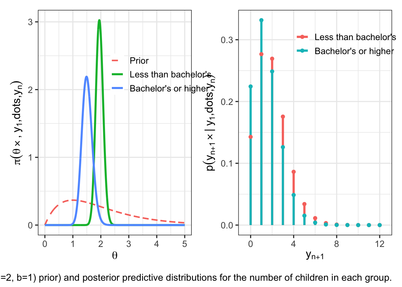

y <- 0:10

Group 1: Less than bachelor's

size = 219   mu = 1.955357

 [1] 1.427473e-01 2.766518e-01 2.693071e-01 1.755660e-01 8.622930e-02
 [6] 3.403387e-02 1.124423e-02 3.198421e-03 7.996053e-04 1.784763e-04
[11] 3.601115e-05


Group 2: Bachelor's or higher

size = 68   mu = 1.511111

 [1] 2.243460e-01 3.316420e-01 2.487315e-01 1.261681e-01 4.868444e-02
 [6] 1.524035e-02 4.030961e-03 9.263700e-04 1.887982e-04 3.465861e-05
[11] 5.801551e-06

    y Less.than.bachelor.s Bachelor.s.or.higher
1   0         1.427473e-01         2.243460e-01
2   1         2.766518e-01         3.316420e-01
3   2         2.693071e-01         2.487315e-01
4   3         1.755660e-01         1.261681e-01
5   4         8.622930e-02         4.868444e-02
6   5         3.403387e-02         1.524035e-02
7   6         1.124423e-02         4.030961e-03
8   7         3.198421e-03         9.263700e-04
9   8         7.996053e-04         1.887982e-04
10  9         1.784763e-04         3.465861e-05
11 10         3.601115e-05         5.801551e-06

Interpretation and Conclusion

Although the posterior distributions of \(\theta_1\) and \(\theta_2\) are clearly separated, the posterior predictive distributions for \(\tilde{Y}_1\) and \(\tilde{Y}_2\) exhibit substantial overlap.

For example,

\[ \Pr(\tilde{Y}_1 > \tilde{Y}_2 \mid y) \approx 0.48, \qquad \Pr(\tilde{Y}_1 = \tilde{Y}_2 \mid y) \approx 0.22. \]

This illustrates an important distinction:

Strong evidence that population means differ does not imply that the difference is large or easily detectable at the individual level.

Note

Population-level effects and individual-level variability are fundamentally different sources of uncertainty.

3.7 Exponential Family

Many common sampling models belong to the exponential family of distributions, including the binomial and Poisson distribution we saw in this chapter. A one-parameter exponential family has probability density (or mass) function of the form \[ \begin{aligned} p(y \mid \phi) &= h(y) \exp\{ \phi t(y) - A(\phi) \} \\ &= h(y) c(\phi) \exp\{\phi t(y)\}, \end{aligned} \] where \(\phi\) is the unknown parameter, \(t(y)\) is a sufficient statistic, and \(h(y)\), \(A(\phi)\), and \(c(\phi)\) are known functions. Diaconis and Ylvisaker (1979) studied conjugate priors for exponential family models and showed that they have the general form \[ p(\phi \mid n_0, t_0) = \kappa (n_0,t_0) c(\phi)^{n_0} \exp \{n_0t_0 \phi\}, \] where \(n_0 > 0\) and \(t_0\) are hyperparameters.

With this result, and suppose the data consist of \(n\) independent observations \(y_1,\ldots,y_n\) are sampled from \(Y_1,\dots,Y_n \stackrel{iid}{\sim} p(y\mid \theta)\). Combining the prior with the likelihood gives the posterior distribution \[ p(\phi \mid y_1, \ldots, y_n) \;\propto\; p(\phi)\, p(y_1, \ldots, y_n \mid \phi). \]

Substituting the exponential-family form, \[ \begin{aligned} p(\phi \mid y_1, \ldots, y_n) &\propto c(\phi)^{\,n_0+n} \exp\left\{ \phi \left[ n_0 t_0 + \sum_{i=1}^n t(y_i) \right] \right\} \\ &\propto p\!\left(\phi \mid n_0 + n,\; n_0 t_0 + n \,\bar t(y)\right), \end{aligned} \] where \[ \bar t(y) = \frac{1}{n}\sum_{i=1}^n t(y_i). \]

Thus, the posterior distribution has the same functional form as the prior. This is why such priors are called conjugate.

3.7.1 Interpretation of \(n_0\) and \(t_0\)

The similarity between the prior and posterior distributions suggests an interpretation of the hyperparameters:

\(n_0\) can be interpreted as a prior sample size,
\(t_0\) can be interpreted as a prior guess of \(t(Y)\).

This interpretation can be made more precise. Diaconis and Ylvisaker (1979) show that \[ \mathbb{E}[t(Y)] = \mathbb{E}\!\left[\,\mathbb{E}[t(Y)\mid \phi]\,\right] = \mathbb{E}\!\left[-\frac{c'(\phi)}{c(\phi)}\right] = t_0. \] (See also Exercise 3.6 in Hopf, 2009)

Thus, \(t_0\) represents the prior expected value of the sufficient statistic \(t(Y)\).

The parameter \(n_0\) measures how informative the prior is. One way to see this is to note that, as a function of \(\phi\), \(p(\phi \mid n_0, t_0)\) has the same shape as a likelihood \(p(\tilde y_1, \ldots, \tilde y_{n_0} \mid \phi)\) based on \(n_0\) hypothetical “prior observations” \(\tilde y_1, \ldots, \tilde y_{n_0}\) satisfying \[ \frac{1}{n_0}\sum_{i=1}^{n_0} t(\tilde y_i) = t_0. \]

In this sense, the prior distribution \(p(\phi \mid n_0, t_0)\) contains the same amount of information as would be obtained from \(n_0\) independent observations from the population.

The exponential family representation of the binomial\((\theta)\) model can be obtained from the density of a single Bernoulli random variable:

\[ p(y \mid \theta) = \theta^y (1-\theta)^{1-y}. \]

Rewrite this as

\[ \begin{aligned} p(y \mid \theta) &= \left( \frac{\theta}{1-\theta} \right)^y (1-\theta) \\ &= \exp\left\{ y \log\left( \frac{\theta}{1-\theta} \right) \right\} (1-\theta). \end{aligned} \]

Let

\[ \phi = \log\left( \frac{\theta}{1-\theta} \right), \]

the log-odds. Then

\[ \theta = \frac{e^\phi}{1+e^\phi}, \qquad 1-\theta = \frac{1}{1+e^\phi}. \]

Substituting gives

\[ p(y \mid \phi) = e^{\phi y} (1+e^\phi)^{-1}. \]

Thus the Bernoulli model is an exponential family model with

\(t(y) = y\),
\(c(\phi) = (1+e^\phi)^{-1}\),
\(h(y) = 1\).

Conjugate prior

The conjugate prior for \(\phi\) has the form

\[ p(\phi \mid n_0, t_0) \propto (1+e^\phi)^{-n_0} \exp\{ n_0 t_0 \phi \}. \]

Since \(t(y)=y\), the parameter \(t_0\) represents the prior expectation of \(Y\), or equivalently,

\[ t_0 = \mathbb{E}(\theta). \]

Using a change of variables back to \(\theta\), the prior becomes

\[ p(\theta \mid n_0, t_0) \propto \theta^{n_0 t_0 - 1} (1-\theta)^{n_0 (1-t_0) - 1}, \]

which is a Beta distribution:

\[ \theta \sim \text{Beta}(n_0 t_0,\; n_0(1-t_0)). \]

A weakly informative prior can be obtained by setting

\(t_0\) equal to our prior expectation,
\(n_0 = 1\).

For example, if our prior expectation is \(1/2\), this gives

\[ \theta \sim \text{Beta}(1/2, 1/2), \]

which is Jeffreys’ prior for the binomial model.

Under this prior, the posterior distribution is

\[ \theta \mid y_1, \ldots, y_n \sim \text{Beta} \left( t_0 + \sum y_i, \; (1-t_0) + \sum (1-y_i) \right). \]

The Poisson\((\theta)\) model can also be written in exponential family form.

The Poisson pmf is

\[ p(y \mid \theta) = \frac{\theta^y e^{-\theta}}{y!}. \]

Rewrite as

\[ p(y \mid \theta) = \frac{1}{y!} \exp\{ y \log\theta - \theta \}. \]

Thus it is an exponential family with

\(t(y) = y\),
\(\phi = \log\theta\),
\(c(\phi) = \exp(-e^\phi)\),
\(h(y) = 1/y!\).

Conjugate prior

The conjugate prior for \(\phi\) has the form

\[ p(\phi \mid n_0, t_0) \propto \exp\{ n_0 t_0 \phi - n_0 e^\phi \}. \]

Transforming back to \(\theta = e^\phi\), this becomes

\[ p(\theta \mid n_0, t_0) \propto \theta^{n_0 t_0 - 1} e^{-n_0 \theta}, \]

which is a Gamma distribution:

\[ \theta \sim \text{Gamma}(n_0 t_0,\; n_0). \]

A weakly informative prior can be obtained by setting

\(t_0\) equal to the prior expectation of \(\theta\),
\(n_0 = 1\),

giving

\[ \theta \sim \text{Gamma}(t_0, 1). \]

Under this prior, the posterior distribution is

\[ \theta \mid y_1, \ldots, y_n \sim \text{Gamma} \left( t_0 + \sum y_i, \; n_0 + n \right). \]

3.8 Discussion

The notion of conjugacy for classes of prior distributions was developed in Raiffa and Schlaifer (1961). Important results on conjugacy for exponential families appear in Diaconis and Ylvisaker (1979) and Diaconis and Ylvisaker (1985). They show that any prior distribution may be approximated by a mixture of conjugate priors.

Most authors refer to intervals of high posterior probability as credible intervals, as opposed to confidence intervals. However, credible intervals do not necessarily have frequentist coverage properties. In many common models they are numerically similar to classical intervals, but this is not guaranteed.

Some authors argue that accurate frequentist coverage can guide the construction of prior distributions. See Kass and Wasserman (1996) for a review of formal methods for selecting prior distributions.

This Chapter follows closely with Chapter 3 in Hoff (2009).