4 Monte Carlo Methods

Leading objectives:

understand how Monte Carlo (MC) and Markov chain Monte Carlo (MCMC) methods differ

learn how to use MC methods to approximate posterior expectations and probabilities

understand how to sample from the posterior predictive distribution using MC methods

What we have seen in the last chapter up to now, is to use the conjugate prior to obtain closed form expressions for the posterior distribution. However, in many cases, conjugate priors are not available or not desirable. In such cases, we need to resort to numerical methods to approximate the posterior distribution.

Question.

How can we perform Bayesian inference when conjugate priors are not available and the posterior has no closed-form expression?

There are two broad classes of approaches:

Simulation-based methods:
accept–reject sampling, Markov chain Monte Carlo (MCMC), particle filters, and related algorithms.
Deterministic approximation methods:
Laplace approximations (including INLA), variational Bayes, expectation propagation, and related techniques.

We will be focusing on the Monte Carlo (MC) methods and its variation.

4.1 Overview

Monte Carlo

MC methods approximate expectations or probabilities using random sampling.

If samples can be drawn directly from the target distribution, Monte Carlo methods provide simple and effective estimators.

Typical use:

Numerical integration
Bootstrap methods
Simulation-based probability estimation

Markov Chain Monte Carlo

MCMC methods are used when direct sampling is infeasible. They construct a Markov chain whose stationary distribution is the target distribution, and use dependent samples from the chain after burn-in.

Typical use:

Bayesian posterior sampling
High-dimensional or unnormalized distributions

Gibbs Sampler

The Gibbs sampler is a special case of MCMC that samples sequentially from full conditional distributions. Because proposals are drawn exactly from conditionals, all updates are automatically accepted.

Typical use:

Bayesian hierarchical models
Models with conjugate full conditionals

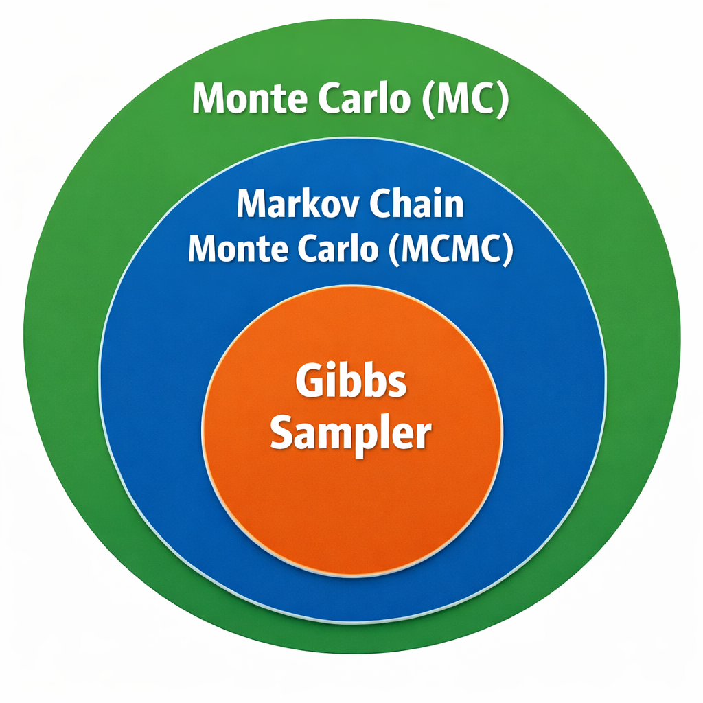
4.1.1 Relationship Between Monte Carlo, MCMC, and Gibbs Sampling

These three concepts are not competing methods, but rather form a nested hierarchy of ideas used for approximating expectations and probability distributions using randomness.

4.1.2 Summary Table

Method	Independent Samples	Uses Markov Chain	Accept–Reject Step	Typical Application
Monte Carlo	Yes	No	No	Direct simulation, integration
MCMC	No	Yes	Usually	Bayesian posterior sampling
Gibbs Sampler	No	Yes	No (always accept)	Bayesian models with tractable conditionals

Key summary

MC is the general idea of using randomness for approximation.
MCMC is MC with dependent samples generated by a Markov chain.
Gibbs sampling is a specific MCMC algorithm based on full conditional distributions.

4.2 Monte Carlo Method

In the previous chapter, we obtained the following posterior distributions for the birth rates of women without and with bachelor’s degrees:

\[ \theta_1 \mid \sum_{i=1}^{111} Y_{i,1} = 217 \sim \text{Gamma}(219, 112), \]

\[ \theta_2 \mid \sum_{i=1}^{44} Y_{i,2} = 66 \sim \text{Gamma}(68, 45). \]

It was claimed that

\[ \Pr(\theta_1 > \theta_2 \mid \text{data}) = 0.97. \]

How do we compute such a probability? From the previous chapter, since \(\theta_1\) and \(\theta_2\) are conditionally independent given the data \(y\), we have \[ \Pr(\theta_1 > \theta_2 \mid y) = \int_0^\infty \int_0^{\theta_1} p(\theta_1 \mid y) p(\theta_2 \mid y) \, d\theta_2 \, d\theta_1. \]

Substituting the gamma densities gives

\[ \int_0^\infty \int_0^{\theta_1} \text{dgamma}(\theta_1; 219, 112) \, \text{dgamma}(\theta_2; 68, 45) \, d\theta_2 \, d\theta_1. \]

This integral can be evaluated numerically. However, in realistic Bayesian models, such integrals quickly become high-dimensional and analytically intractable. This motivates Monte Carlo (MC) methods.

In Bayesian inference we repeatedly encounter integrals such as

\[ \mathbb{E}[g(\theta)\mid y] =\int g(\theta)\,p(\theta\mid y)\,d\theta, \qquad \Pr(\theta\in A\mid y)=\int_A p(\theta\mid y)\,d\theta, \]

that are not available in closed form. MC replaces these integrals by averages of random draws.

Key Idea

Replace an intractable integral by an empirical mean.

4.2.1 MC Approximation

Suppose we wish to compute

\[ \mathbb{E}[g(\theta) \mid y] = \int g(\theta) \, p(\theta \mid y) \, d\theta. \]

If we can generate independent samples

\[ \theta^{(1)}, \ldots, \theta^{(S)} \sim p(\theta \mid y), \]

then we approximate the expectation by

\[ \frac{1}{S} \sum_{s=1}^S g(\theta^{(s)}). \]

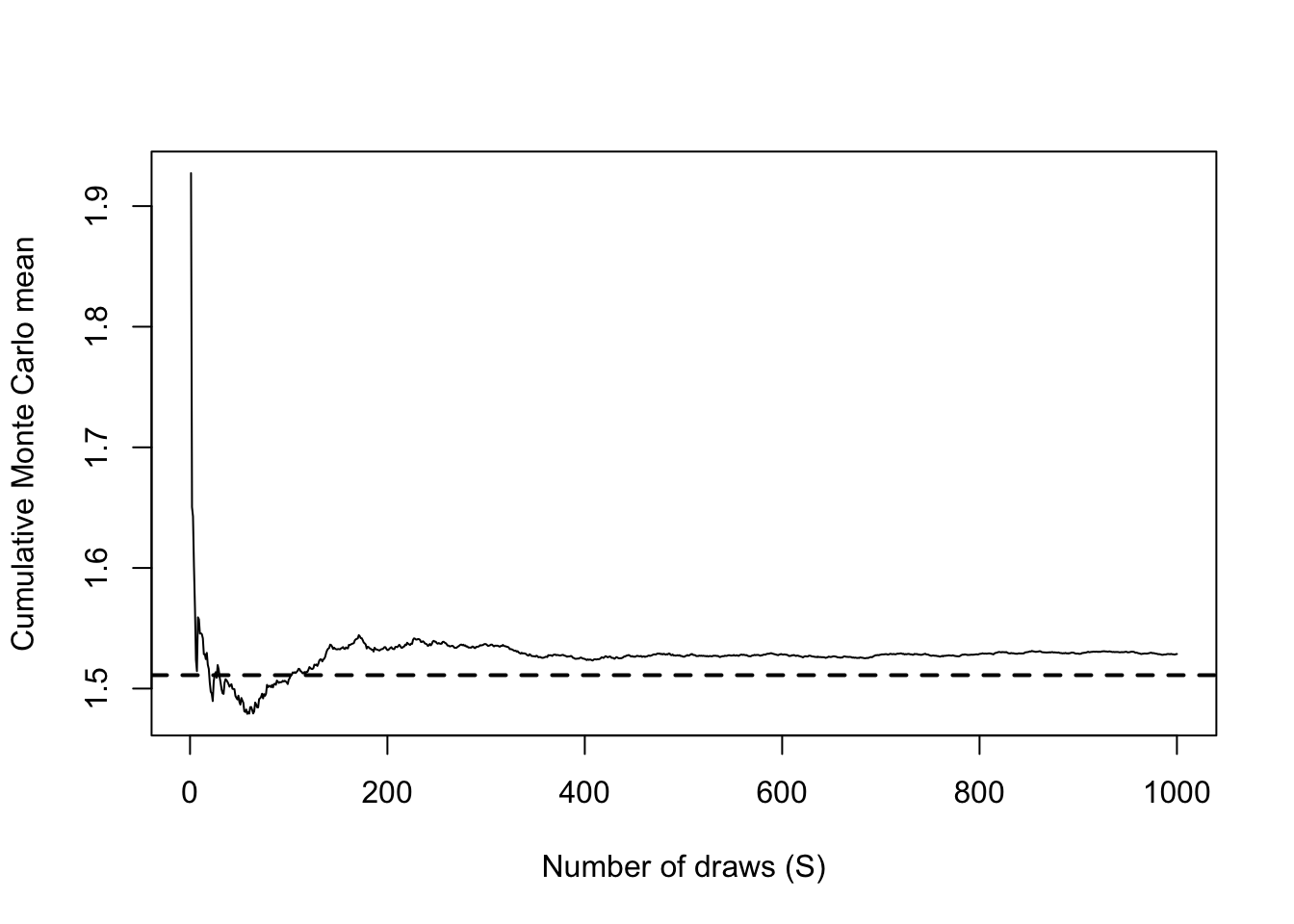
This is called a Monte Carlo approximation. By the Law of Large Numbers,

\[ \frac{1}{S} \sum_{s=1}^S g(\theta^{(s)}) \;\longrightarrow\; \mathbb{E}[g(\theta) \mid y] = \int g(\theta) p(\theta \mid y) d\theta \quad \text{as } S \to \infty. \] With the property above, we can calculate many quantities of interest about the posterior distribution. For example, suppose \(\bar{\theta}\) is the average of \(\{\theta^{(1)}, \dots, \theta^{(S)}\}\), then as \(S \to \infty\):

\(\bar{\theta} \to \mathbb{E}[\theta \mid y]\),
\(\frac{1}{S-1}\sum_{s=1}^S (\theta^{(s)} - \bar{\theta})^2\to \mathrm{Var}(\theta \mid y)\).
\(\frac{1}{S}\sum_{s=1}^S \mathbf{1}\{\theta^{(s)} \in A\}\to \Pr(\theta \in A \mid y)\).
the empirical distribution of \(\{\theta^{(1)}, \dots, \theta^{(S)}\}\) converges to \(p(\theta \mid y)\).
the sample median converges to the posterior median \(\theta_{1/2}\).
the sample \(\alpha\)-quantile converges to \(\theta_\alpha\).

Key message

Almost any aspect of a posterior distribution can be approximated arbitrarily well using a sufficiently large Monte Carlo sample.

working in high dimensions
requires only the ability to simulate
avoids symbolic integration.
Scales to complex hierarchical models.

Thus Monte Carlo sampling allows us to approximate:

posterior means,
posterior variances,
posterior probabilities,
credible intervals,
many more

To approximate \[ \Pr(\theta_1 > \theta_2 \mid y), \]

we can:

Choose a (large) number of samples \(S\) (e.g., \(S=10,000\)).
Draw \(\theta_1^{(s)} \sim \text{Gamma}(219, 112)\).
Draw \(\theta_2^{(s)} \sim \text{Gamma}(68, 45)\).
Compute the indicator \[ I^{(s)} = \mathbf{1}\{\theta_1^{(s)} > \theta_2^{(s)}\}. \]

Then

\[ \Pr(\theta_1 > \theta_2 \mid y) \approx \frac{1}{S} \sum_{s=1}^S I^{(s)}. \]

This avoids evaluating any double integrals. This is the foundation of modern Bayesian computation.

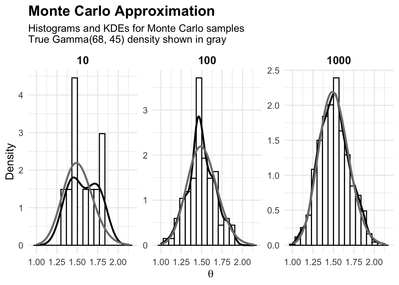
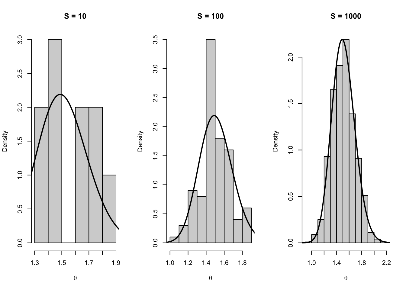
# Figure 4.1 — Monte Carlo Approximation (Gamma(68,45))
# Histograms + KDEs for S = 10, 100, 1000; true density in gray

set.seed(8310)
library(ggplot2)

# Posterior: Gamma(shape=68, rate=45)
shape_post <- 68
rate_post  <- 45

# MC samples
S_list <- c(10, 100, 1000)
mc_df <- do.call(rbind, lapply(S_list, function(S) {
  data.frame(theta = rgamma(S, shape = shape_post, rate = rate_post),
             S = factor(S, levels = S_list))
}))

# Grid for true density (choose a sensible range around the mass)
xgrid <- seq(
  qgamma(0.001, shape = shape_post, rate = rate_post),
  qgamma(0.999, shape = shape_post, rate = rate_post),
  length.out = 600
)

true_df <- data.frame(
  theta = xgrid,
  dens  = dgamma(xgrid, shape = shape_post, rate = rate_post)
)

# Plot
ggplot(mc_df, aes(x = theta)) +
  # histogram (density scale so it overlays with densities)
  geom_histogram(aes(y = after_stat(density)),
                 bins = 18, color = "black", fill = "white") +
  # KDE from MC samples
  geom_density(linewidth = 1.1) +
  # True density (gray)
  geom_line(data = true_df, aes(x = theta, y = dens),
            linewidth = 1.2, color = "gray50") +
  facet_wrap(~ S, nrow = 1, scales = "free_y") +
  labs(
    title = "Monte Carlo Approximation",
  subtitle = paste(
    "Histograms and KDEs for Monte Carlo samples",
    "True Gamma(68, 45) density shown in gray",
    sep = "\n"
  ),
    x = expression(theta),
    y = "Density"
  ) +
  theme_minimal(base_size = 14) +
  theme(
    plot.title = element_text(size = 18, face = "bold"),
    plot.subtitle = element_text(size = 13),
    strip.text = element_text(size = 14, face = "bold")
  )

4.2.1.1 Numerical Evaluation

We now compare MC approximations to quantities that can be computed analytically in this conjugate example.

Suppose

\[ Y_1,\dots,Y_n \mid \theta \sim \text{Poisson}(\theta), \quad \theta \sim \text{Gamma}(a,b). \]

After observing \(y_1,\dots,y_n\) with \(\sum y_i = sy\) and sample size \(n\), the posterior distribution is

\[ \theta \mid y \sim \text{Gamma}(a+sy,\; b+n). \]

For the birth-rate example:

\(a = 2\)
\(b = 1\)
\(sy = 66\)
\(n = 44\)

Posterior:

\[ \theta \mid y \sim \text{Gamma}(68,45). \]

Posterior mean:

\[ \mathbb{E}[\theta \mid y] = \frac{a+sy}{b+n} = \frac{68}{45} = 1.51. \]

set.seed(8310)

## Posterior parameters
a  <- 2
b  <- 1
sy <- 66
n  <- 44

shape_post <- a + sy
rate_post  <- b + n

## Exact quantities
mean_exact <- shape_post / rate_post
p_exact    <- pgamma(1.75, shape = shape_post, rate = rate_post)
ci_exact   <- qgamma(c(0.025, 0.975),
                     shape = shape_post,
                     rate  = rate_post)

## Monte Carlo samples
theta_mc10   <- rgamma(10,   shape_post, rate_post)
theta_mc100  <- rgamma(100,  shape_post, rate_post)
theta_mc1000 <- rgamma(1000, shape_post, rate_post)

## Function to summarize MC output
mc_summary <- function(theta_sample) {
  c(
    Mean        = mean(theta_sample),
    Prob_less   = mean(theta_sample < 1.75),
    CI_lower    = quantile(theta_sample, 0.025),
    CI_upper    = quantile(theta_sample, 0.975)
  )
}

## Build comparison table
results <- rbind(
  Exact   = c(Mean      = mean_exact,
              Prob_less = p_exact,
              CI_lower  = ci_exact[1],
              CI_upper  = ci_exact[2]),

  MC_10   = mc_summary(theta_mc10),
  MC_100  = mc_summary(theta_mc100),
  MC_1000 = mc_summary(theta_mc1000)
)

round(results, 4)

          Mean Prob_less CI_lower CI_upper
Exact   1.5111    0.8998   1.1734   1.8908
MC_10   1.5782    0.8000   1.3408   1.8149
MC_100  1.4968    0.9300   1.1801   1.8349
MC_1000 1.5102    0.8850   1.1578   1.8817

Smax <- 1000
theta_seq <- rgamma(Smax, shape = shape_post, rate = rate_post)
cum_mean  <- cumsum(theta_seq) / seq_along(theta_seq)

plot(cum_mean, type="l",
     xlab="Number of draws (S)",
     ylab="Cumulative Monte Carlo mean")
abline(h = mean_exact, lty = 2, lwd = 2)

xgrid <- seq(0.5, 2.5, length.out = 400)
true_pdf <- dgamma(xgrid, shape = shape_post, rate = rate_post)

par(mfrow=c(1,3))

for (S in c(10,100,1000)) {
  x <- get(paste0("theta_mc", S))
  hist(x, prob=TRUE,
       main=paste0("S = ", S),
       xlab=expression(theta),
       border="black")
  lines(xgrid, true_pdf, lwd=2)
}

MC offers much more

There are much more about the MC method**

Variance reduction methods
Antithetic variates
Control variables
Importance Sampling
Stratified Sampling
Stratified Importance Sampling
etc…

You may refer to my notes in Chapter 4 in the Computational Methods in Statistics Course.

4.2.2 MC for predictive distribution and Sampling from it

As discussed earlier, the predictive distribution of a future random variable \(\tilde Y\) is the probability distribution that reflects uncertainty about \(\tilde Y\) after accounting for both:

known quantities (conditioned on observed data), and
unknown quantities (integrated out).

4.2.2.1 Sampling Model vs Predictive Model

Suppose \(\tilde Y\) denotes the number of children for a randomly selected woman aged 40 with a college degree.

If the true mean birthrate \(\theta\) were known, uncertainty about \(\tilde Y\) would be described by the sampling model \[ \Pr(\tilde Y = \tilde y \mid \theta) = p(\tilde y \mid \theta) = \frac{\theta^{\tilde y} e^{-\theta}}{\tilde y!}, \] that is, \[ \tilde Y \mid \theta \sim \text{Poisson}(\theta). \]

In practice, however, \(\theta\) is unknown. Therefore, predictions must account for uncertainty in \(\theta\).

4.2.2.2 Prior Predictive Distribution

If no data have been observed, predictions are obtained by integrating out \(\theta\) using the prior distribution: \[ \Pr(\tilde Y = \tilde y) = \int p(\tilde y \mid \theta)\, p(\theta)\, d\theta. \]

This is called the prior predictive distribution.

For a Poisson model with a Gamma prior, \[ \theta \sim \text{Gamma}(a,b), \] the prior predictive distribution of \(\tilde Y\) is \[ \tilde Y \sim \text{Negative Binomial}(a,b). \]

4.2.2.3 Posterior Predictive Distribution

After observing data \(Y_1 = y_1, \ldots, Y_n = y_n\), the relevant predictive distribution for a new observation is \[ \Pr(\tilde Y = \tilde y \mid Y_1=y_1,\ldots,Y_n=y_n) = \int p(\tilde y \mid \theta)\, p(\theta \mid y_1,\ldots,y_n)\, d\theta. \]

This distribution is called the posterior predictive distribution.

For the Poisson–Gamma model, the posterior distribution is \[ \theta \mid y_1,\ldots,y_n \sim \text{Gamma}\!\left(a + \sum_{i=1}^n y_i,\; b+n\right), \] and the posterior predictive distribution is again Negative Binomial.

4.2.2.4 MC Sampling from the Posterior Predictive Distribution

In many models, the posterior predictive distribution cannot be evaluated analytically. However, it can often be sampled using MC methods.

The idea is simple:

Draw \(\theta^{(s)} \sim p(\theta \mid y_1,\ldots,y_n)\)
Draw \(\tilde Y^{(s)} \sim p(\tilde y \mid \theta^{(s)})\)
Repeat for \(s = 1,\ldots,S\)

This produces samples \[ \tilde Y^{(1)}, \ldots, \tilde Y^{(S)} \sim p(\tilde y \mid y_1,\ldots,y_n), \] which approximate the posterior predictive distribution.

Suppose we observe two independent groups with Poisson data:

Group 1: \(\sum Y_{i,1} = 217\), \(n_1 = 111\)
Group 2: \(\sum Y_{i,2} = 66\), \(n_2 = 44\)

With a common prior \[ \theta_k \sim \text{Gamma}(a,b), \quad k=1,2, \] the posterior distributions are \[ \theta_1 \mid \mathbf y_1 \sim \text{Gamma}(a+217,\; b+111), \] \[ \theta_2 \mid \mathbf y_2 \sim \text{Gamma}(a+66,\; b+44). \]

Because \(\theta_1\) and \(\theta_2\) are posterior independent, posterior predictive sampling proceeds independently for each group:

\[ \theta_1^{(s)} \sim p(\theta_1 \mid \mathbf y_1), \quad \tilde Y_1^{(s)} \sim \text{Poisson}(\theta_1^{(s)}), \] \[ \theta_2^{(s)} \sim p(\theta_2 \mid \mathbf y_2), \quad \tilde Y_2^{(s)} \sim \text{Poisson}(\theta_2^{(s)}). \]

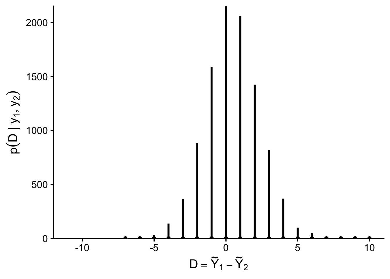
Using Monte Carlo samples \(\{\tilde Y_1^{(s)}, \tilde Y_2^{(s)}\}\), we can approximate quantities such as \[ \Pr(\tilde Y_1 > \tilde Y_2 \mid \text{data}) \approx \frac{1}{S} \sum_{s=1}^S \mathbb{I}\bigl(\tilde Y_1^{(s)} > \tilde Y_2^{(s)}\bigr). \]

More generally, MC samples from the posterior predictive distribution allow us to approximate:

predictive probabilities,
predictive expectations,
quantiles and credible intervals,
functions of future observations.

This flexibility is one of the main strengths of MC methods in Bayesian analysis.

4.3 Posterior inference for arbitrary functions

Often we care about the posterior distribution of some computable function \(g(\theta)\) of a parameter \(\theta\). For example, in the binomial model we may be interested in the log-odds \[ \text{log odds}(\theta) = \log\!\left(\frac{\theta}{1-\theta}\right) = \gamma. \]

If we can generate posterior draws \(\{\theta^{(1)},\theta^{(2)},\ldots\}\) from \(p(\theta\mid y_1,\ldots,y_n)\), then the law of large numbers implies that Monte Carlo averages converge to posterior expectations. For instance, \[ \frac{1}{S}\sum_{s=1}^S \log\!\left(\frac{\theta^{(s)}}{1-\theta^{(s)}}\right) \;\longrightarrow\; \mathbb{E}\!\left[\log\!\left(\frac{\theta}{1-\theta}\right)\middle|y_1,\ldots,y_n\right]. \]

More generally, we can approximate the entire posterior distribution of \[ \gamma = g(\theta) = \log\!\left(\frac{\theta}{1-\theta}\right) \] by transforming posterior samples:

\[ \theta^{(1)} \sim p(\theta\mid y_1,\ldots,y_n), \quad \gamma^{(1)} = g(\theta^{(1)}), \] \[ \theta^{(2)} \sim p(\theta\mid y_1,\ldots,y_n), \quad \gamma^{(2)} = g(\theta^{(2)}), \] \[ \vdots \] \[ \theta^{(S)} \sim p(\theta\mid y_1,\ldots,y_n), \quad \gamma^{(S)} = g(\theta^{(S)}). \]

The collection \(\{\gamma^{(1)},\ldots,\gamma^{(S)}\}\) approximates the posterior distribution of \(\gamma\), so we can estimate posterior means, variances, quantiles, and credible intervals for \(\gamma\) directly from these transformed draws.

4.3.1 Posterior Predictive Model Checking

library(ggplot2)

set.seed(8670)

## --- Birth-rate example (Hoff): posterior predictive for D = Y~1 - Y~2 ---
a  <- 2;  b  <- 1
n1 <- 111; sy1 <- 217   # less than bachelor's
n2 <- 44;  sy2 <- 66    # bachelor's or higher

shape1 <- a + sy1; rate1 <- b + n1
shape2 <- a + sy2; rate2 <- b + n2

S <- 10000  # using 10,000 makes the y-axis peak around ~2000 (counts), like Fig 4.5

theta1 <- rgamma(S, shape = shape1, rate = rate1)
theta2 <- rgamma(S, shape = shape2, rate = rate2)

y1 <- rpois(S, lambda = theta1)
y2 <- rpois(S, lambda = theta2)

D <- y1 - y2

df <- as.data.frame(table(D))
df$D <- as.integer(as.character(df$D))
df$Freq <- as.numeric(df$Freq)

xlim <- c(-12, 11)

ggplot(df, aes(x = D, y = Freq)) +
  geom_segment(aes(xend = D, y = 0, yend = Freq),
               linewidth = 1.2, color = "black") +
  geom_point(aes(y = 0), size = 1.6, color = "black") +
  coord_cartesian(xlim = xlim, expand = FALSE) +
  labs(
    x = expression(D == tilde(Y)[1] - tilde(Y)[2]),
    y = expression(p(D~"|"~y[1],y[2]))
  ) +
  theme_classic(base_size = 16)

Posterior predictive model checking assesses whether a fitted Bayesian model can plausibly reproduce key features of the observed data. Back to the example we studied before, we focus on women aged 40 without a college degree. The empirical distribution of the number of children for these women, together with the corresponding posterior predictive distribution.

In this sample of size \(n = 111\), the number of women with exactly two children is \(y_{\text{obs}} = 38,\) which is twice the number of women with exactly one child.

In contrast, the posterior predictive distribution (shown in gray) suggests that sampling a woman with two children is slightly less likely than sampling a woman with one child, with probabilities approximately \[ 0.27 \quad \text{vs.} \quad 0.28. \]

These two distributions appear to be in conflict: if the observed data contain twice as many women with two children as with one child, why does the model predict otherwise?

Possible Explanations

One explanation is sampling variability. The empirical distribution of a finite sample does not necessarily match the true population distribution, and with moderate sample sizes, random fluctuations can be substantial. A smooth population distribution can easily produce a bumpy empirical histogram.

An alternative explanation is model misspecification. In particular, the Poisson model cannot capture certain features of the data. There is no Poisson distribution with a sharp peak at \(y = 2\), whereas the empirical distribution shows exactly such behaviour.

These explanations can be investigated systematically using Monte Carlo simulation. Define the discrepancy statistic \[ t(y) = \frac{\#{y_i = 2}}{\#{y_i = 1}}, \] the ratio of the number of women with two children to the number with one child.

For the observed data, \(t(y_{\text{obs}}) = 2.\) To assess whether this value is surprising under the model, we examine the posterior predictive distribution of \(t(\tilde{Y})\).

For each Monte Carlo iteration \(s = 1, \dots, S\):

Sample from the posterior \[\theta^{(s)} \sim p(\theta \mid y_{\text{obs}})\]
Generate a posterior predictive dataset \[\tilde{Y}^{(s)} = (\tilde{y}_1^{(s)}, \dots, \tilde{y}_n^{(s)}), \quad \text{where } \tilde{y}_i^{(s)} \stackrel{\text{i.i.d.}}{\sim} \text{Poisson}(\theta^{(s)})\]
Compute the discrepancy \[t^{(s)} = t(\tilde{Y}^{(s)})\]

This yields samples \(\{ t^{(1)}, \dots, t^{(S)} \}\) from the posterior predictive distribution of \(t(\tilde{Y})\).

## Prior parameters
a <- 2
b <- 1

## Data summary (no bachelor's degree group)
n  <- 111
sy <- 217   # sum(y_i)

## Storage
t_mc <- numeric(10000)
set.seed(8310)
for (s in 1:10000) {
  ## Draw from posterior
  theta <- rgamma(1, shape = a + sy, rate = b + n)
  
  ## Posterior predictive sample
  y_mc <- rpois(n, theta)
  
  ## Discrepancy statistic
  n1 <- sum(y_mc == 1)
  n2 <- sum(y_mc == 2)
  
  ## Avoid division by zero
  t_mc[s] <- ifelse(n1 > 0, n2 / n1, NA)
}

## Remove undefined values
t_mc <- t_mc[!is.na(t_mc)]
library(tibble)
library(tibble)
library(knitr)

summary_table <- tibble(
  Quantity = c(
    "Number of valid posterior predictive draws",
    "Number of draws with T ≥ 2.0",
    "Posterior predictive probability P(T ≥ 2.0)"
  ),
  Value = c(
    format(length(t_mc), big.mark = ","),
    format(sum(t_mc >= 2.0), big.mark = ","),
    formatC(mean(t_mc >= 2.0), format = "f", digits = 4)
  )
)

kable(
  summary_table,
  align = c("l", "r"),
  caption = "Posterior Predictive Summary for Discrepancy Statistic T"
)

Posterior Predictive Summary for Discrepancy Statistic T
Quantity	Value
Number of valid posterior predictive draws	10,000
Number of draws with T ≥ 2.0	71
Posterior predictive probability P(T ≥ 2.0)	0.0071

library(ggplot2)

df <- data.frame(t = t_mc)

ggplot(df, aes(x = t)) +
  geom_histogram(
    aes(y = after_stat(count)),
    bins = 40,
    fill = "grey80",
    color = "black"
  ) +
  geom_vline(
    xintercept = 2,
    linewidth = 1,
    linetype = "dashed",
    color = "red"
  ) +
  labs(
    title = "Posterior Predictive Distribution of Discrepancy Statistic",
    subtitle = expression(
      t == frac("#(Y = 2)", "#(Y = 1)")
    ),
    x = expression(t),
    y = "Frequency"
  ) +
  theme_minimal(base_size = 13)

This Figure shows the posterior predictive distribution of \(t(\tilde{Y})\), with the observed value \(t(y_{\text{obs}})=2\) indicated by a vertical line. Out of 10,000 Monte Carlo samples, only about 0.71% produce values of \[ t(\tilde{Y}) \ge t(y_{\text{obs}}). \]

This indicates that the observed discrepancy is extremely unlikely under the fitted Poisson model.

Conclusion

The posterior predictive check suggests that the Poisson model is inadequate for these data. Although it matches the posterior mean reasonably well, it fails to reproduce important distributional features.

This does not imply that the model is useless for all inferential goals. However, if our goal is to accurately describe the distribution of family sizes, a more flexible model is needed.

Posterior predictive checks provide a principled, simulation-based tool for diagnosing such failures and guiding model refinement.

This Chapter borrows materials from Chapter 4 in Hoff (2009) and Chapter 4 in Computational Methods in Statistics Course