8  Diagnostics and Model Adequacy

In this chapter, we study how to assess whether a fitted linear regression model is adequate. After learning estimation, inference, ANOVA, and interpretation, we now turn to model checking. The main tools are residuals, diagnostic plots, and numerical measures that help identify nonlinearity, unequal variance, outliers, and influential observations.

Learning Objectives

By the end of this chapter, students should be able to:

• explain why model diagnostics are necessary after fitting a regression model;
• define raw, standardized, and studentized residuals;
• interpret residual plots for common types of model failure;
• distinguish between outliers in the response direction and influential observations in the design space;
• use leverage, Cook’s distance, and related diagnostics;
• assess model adequacy using graphical and numerical tools.

Reading

Recommended reading for this chapter:

• Seber and Lee:
  • sections on residual analysis
  • diagnostics for regression models
  • influence and unusual observations
• Montgomery, Peck, and Vining:
  • sections on residuals
  • diagnostic plots
  • outliers, leverage, and influence

Why Diagnostics Matter

A fitted regression model may look statistically significant and still be inappropriate. For example:

• the relationship may not be linear;
• the error variance may not be constant;
• the error distribution may be strongly non-normal;
• a small number of unusual observations may dominate the fit.

So regression analysis does not end when we obtain estimates and \(p\)-values. We must also ask whether the model assumptions are reasonable and whether the fit is being driven by problematic observations.

Review of the Linear Model Assumptions

Recall the classical linear model

\[ \mathbf{Y} = \mathbf{X}\boldsymbol{\beta} + \boldsymbol{\varepsilon}, \]

with assumptions such as

\[ \mathbb{E}[\boldsymbol{\varepsilon}] = \mathbf{0}, \qquad \mathrm{Var}(\boldsymbol{\varepsilon}) = \sigma^2 \mathbf{I}_n. \]

Under the normal linear model, we also assume

\[ \boldsymbol{\varepsilon} \sim N_n(\mathbf{0}, \sigma^2 \mathbf{I}_n). \]

These assumptions support:

• unbiasedness of OLS;
• standard error formulas;
• \(t\) and \(F\) inference;
• prediction intervals.

Diagnostics help us investigate whether these assumptions seem plausible for the observed data.

8.1 Residuals

The fitted values are

\[ \hat{\mathbf{Y}} = \mathbf{X}\hat{\boldsymbol{\beta}}, \]

and the residual vector is

\[ \mathbf{e} = \mathbf{Y} - \hat{\mathbf{Y}}. \]

The \(i\)th residual is

\[ e_i = Y_i - \hat{Y}_i. \]

A residual measures how far an observed response is from the fitted value at that observation. Residuals are the basic raw material of regression diagnostics.

ImportantResiduals are not the true errors

Residuals are not the same as the true errors. The true model error is

\[ \varepsilon_i = Y_i - \mathbb{E}[Y_i \mid \mathbf{x}_i], \]

whereas the residual is

\[ e_i = Y_i - \hat{Y}_i. \]

Residuals are observable, but errors are not. Diagnostics therefore use residuals as proxies for model errors.

Properties of Residuals

From least squares geometry, we know that

\[ \mathbf{X}^\top \mathbf{e} = \mathbf{0}. \]

If the model contains an intercept, then

\[ \sum_{i=1}^n e_i = 0. \]

Thus residuals are constrained and are not independent. This is one reason why it is useful to standardize them before interpretation.

Residual Variance and Leverage

Recall the hat matrix

\[ \mathbf{H} = \mathbf{X}(\mathbf{X}^\top \mathbf{X})^{-1}\mathbf{X}^\top. \]

Its diagonal entries \(h_{ii}\) are called leverages. Under the standard model,

\[ \mathrm{Var}(e_i) = \sigma^2(1-h_{ii}). \]

So residuals do not all have the same variance. Observations with high leverage tend to have smaller residual variance. This is why raw residuals alone can be misleading.

Standardized Residuals

A common adjustment is to divide each residual by its estimated standard deviation. The standardized residual is

\[ r_i = \frac{e_i}{\hat{\sigma}\sqrt{1-h_{ii}}}. \]

This puts residuals on a comparable scale across observations. Large absolute values of \(r_i\) may indicate unusual observations in the response direction.

Studentized Residuals

A more refined version is the studentized residual. One version uses the variance estimate computed from the full model. Another version uses the variance estimate obtained after deleting the \(i\)th observation. The externally studentized residual is often written as

\[ t_i = \frac{e_i}{\hat{\sigma}_{(i)}\sqrt{1-h_{ii}}}, \]

where \(\hat{\sigma}_{(i)}^2\) is the residual variance estimate from the model fit without observation \(i\). These are especially useful for outlier detection.

8.2 Diagnostic Plots

One of the most important diagnostic plots is the plot of residuals versus fitted values. This plot helps detect:

• nonlinearity;
• unequal variance;
• outliers;
• missing structure.

A good residual plot usually shows points randomly scattered around zero with roughly constant spread. Patterns are warning signs.

Interpreting Common Patterns

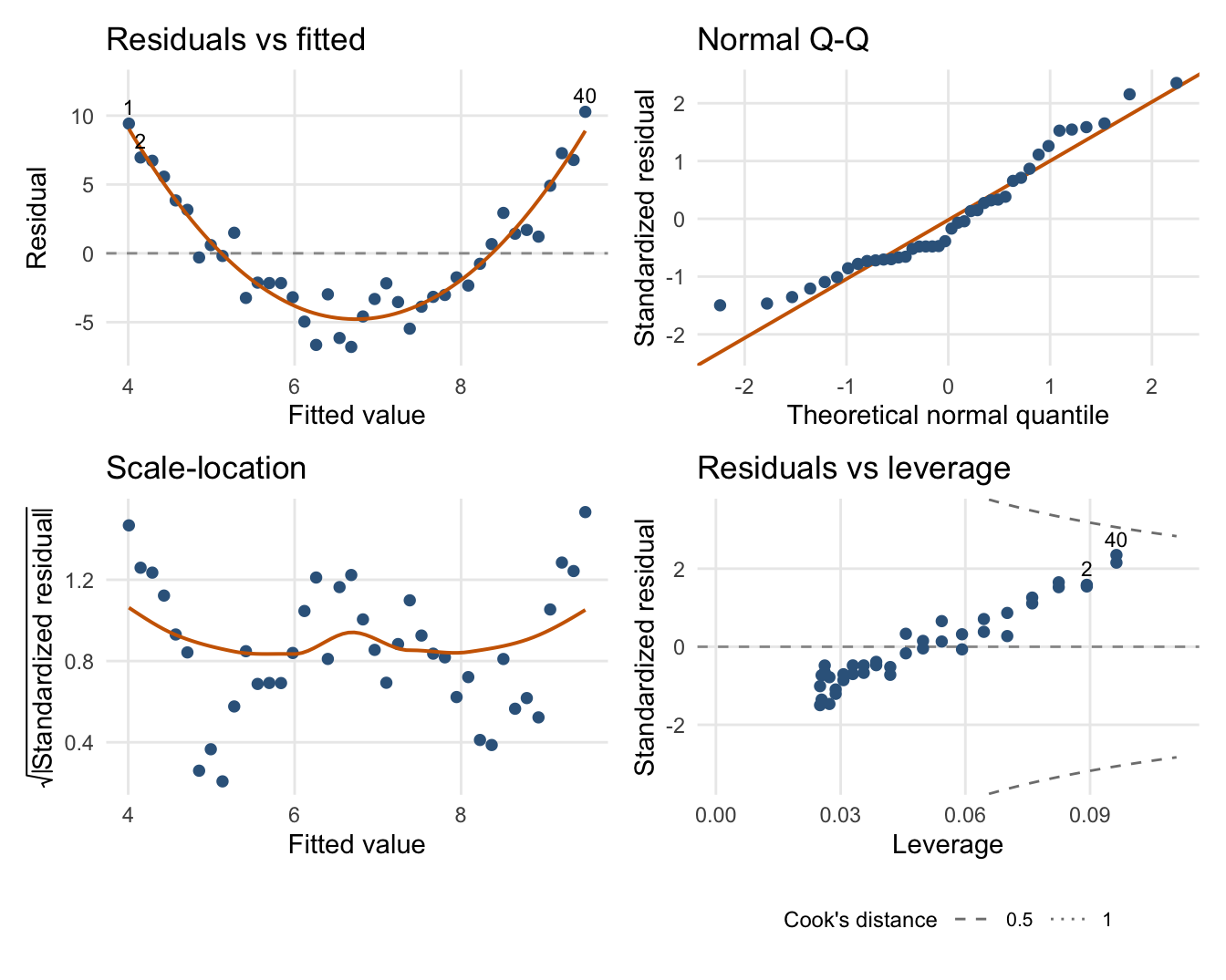
If the residual plot shows a curved pattern, that suggests the mean function may not be adequately linear. If the spread of residuals increases or decreases with the fitted values, that suggests heteroscedasticity, meaning nonconstant error variance. If a few points are isolated far from the rest, they may be outliers or influential observations. Thus the residual plot is often the first and most important diagnostic tool.

Residuals Versus Individual Predictors

It is often helpful to plot residuals against each predictor separately. A residual-versus-predictor plot can reveal:

• nonlinearity in that predictor;
• different spread across ranges of the predictor;
• group-specific patterns;
• possible interactions not included in the model.

These plots are often more informative than a single omnibus diagnostic.

Normal Q-Q Plot

The normal Q-Q plot is used to assess whether the residual distribution is approximately normal. If the normality assumption is reasonable, the residual points should fall approximately along a straight line. Departures from linearity suggest:

• skewness;
• heavy tails;
• light tails;
• extreme outliers.

Normality matters most when sample size is small and exact \(t\) and \(F\) inference is important.

Histogram of Residuals

A histogram of residuals can also be useful, though it is usually less informative than a Q-Q plot. It may reveal:

• skewness;
• multimodality;
• heavy tails;
• extreme asymmetry.

However, the histogram depends strongly on bin choices, so it is usually used as a supplementary plot rather than the main normality diagnostic.

Scale-Location Plot

A scale-location plot often displays \(\sqrt{|r_i|}\) against fitted values. This is another way to assess whether the variance is approximately constant across the fitted range. A roughly horizontal band is desirable. A systematic increase or decrease suggests heteroscedasticity.

Outliers

An outlier is an observation whose response value is unusual relative to the fitted model. In regression, an observation can be outlying in the response direction even if its predictor values are not unusual. Large residuals or large studentized residuals often indicate potential outliers. However, not every outlier is influential.

Leverage

Leverage measures how unusual an observation is in the predictor space. The leverage of observation \(i\) is \(h_{ii}\). High leverage points are far from the center of the predictor cloud in a geometric sense. These points have greater potential to affect the fitted regression line or plane. A rough rule of thumb is that leverage values substantially larger than

\[ \frac{2p}{n} \quad \text{or sometimes} \quad \frac{3p}{n} \]

may deserve attention, where \(p\) is the number of parameters including the intercept. These are only rough guidelines, not formal cutoffs.

Outlier Versus High-Leverage Point

It is important to distinguish between:

• a point with a large residual;
• a point with high leverage.

A point can have:

• low leverage and large residual;
• high leverage and small residual;
• both high leverage and large residual.

The last case is often the most concerning because such a point may strongly influence the fitted model. For additional coefficient-specific and partial-regression diagnostics, see Optional linear-model extensions.

8.3 Influence

An observation is influential if removing it changes the fitted model noticeably. Influence depends on both:

• how unusual the response is;
• how unusual the predictor values are.

So influential points often combine high leverage with a sizable residual. Influence is not the same as being an outlier.

Cook’s Distance

One of the most widely used influence measures is Cook’s distance. Cook’s distance for observation \(i\) measures how much the fitted values change when observation \(i\) is removed. A common formula is

\[ D_i = \frac{e_i^2}{p\hat{\sigma}^2} \cdot \frac{h_{ii}}{(1-h_{ii})^2}. \]

Large values of \(D_i\) indicate potentially influential observations. Plots of Cook’s distance help identify observations that deserve closer inspection.

Diagnosing Nonlinearity

If the mean function is nonlinear but we fit a linear model, residual plots may show curvature. Possible remedies include:

• adding polynomial terms;
• applying transformations;
• including interactions;
• using a different modelling framework.

Diagnostics should not be viewed only as fault-finding. They also guide model improvement.

Diagnosing Heteroscedasticity

If the error variance is not constant, residual plots may show a funnel shape or other changing spread. Possible remedies include:

• transforming the response;
• weighted least squares;
• modelling the variance structure explicitly;
• using heteroscedasticity-robust standard errors in some contexts.

At this stage, the main goal is to recognize the pattern and understand its consequences.

Diagnosing Non-Normality

If residuals are strongly non-normal, this may affect exact small-sample inference. Possible causes include:

• skewed responses;
• heavy-tailed errors;
• outliers;
• omitted structure.

Possible remedies include:

• transformation;
• alternative modelling assumptions;
• robust procedures;
• careful interpretation if sample size is large and inference is approximately stable.

Diagnostics Are Contextual

There is no single diagnostic that automatically declares a model valid or invalid. Instead, diagnostics require judgment. Students should ask:

• Is the pattern strong or mild?
• Is it scientifically meaningful?
• Does one point dominate the fit?
• Would conclusions change if the model were modified?
• Is the issue important for the goal of the analysis: explanation, prediction, or inference?

Worked Example With an Outlying Observation

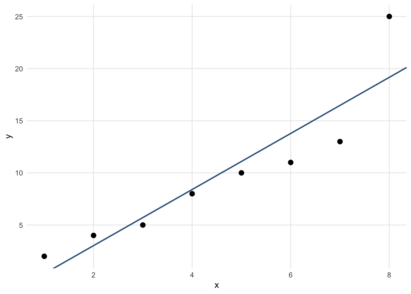
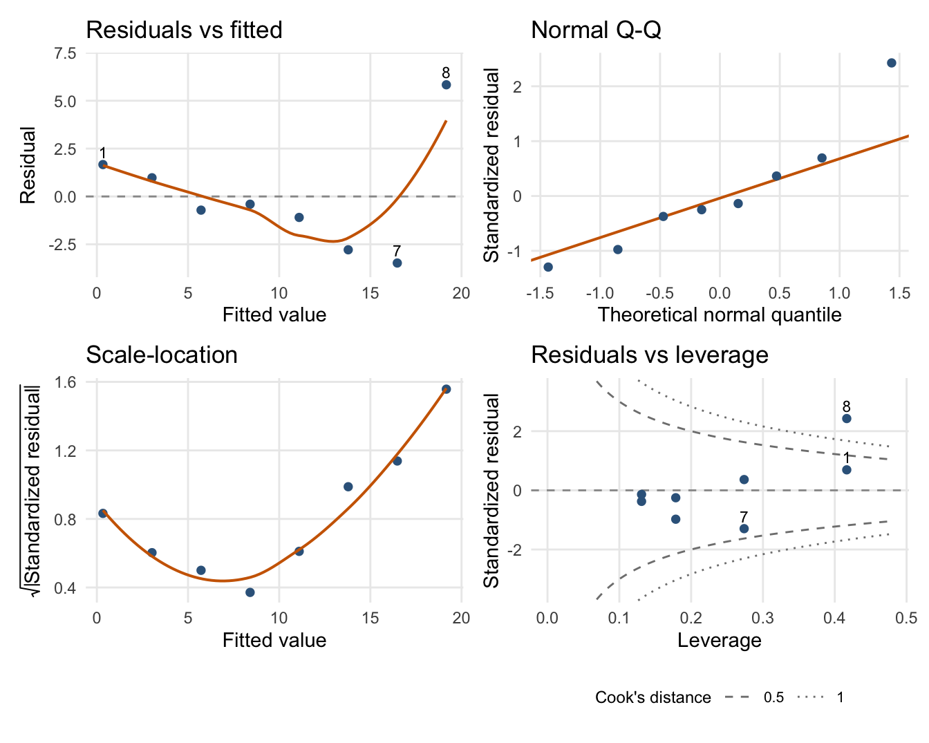
Consider the data \(x = (1,2,3,4,5,6,7,8)\), and \(y = (2,4,5,8,10,11,13,25)\). The final observation may look unusual because the response jumps upward relative to the earlier trend. If we fit a simple linear regression, we should examine:

• the scatterplot with fitted line;
• residuals versus fitted values;
• studentized residuals;
• leverage;
• Cook’s distance.

This is a good example for discussing the difference between an outlier and an influential point.

8.4 R Demonstration

Fit a simple model

library(ggplot2)
theme_set(theme_minimal(base_size = 11) +
            theme(legend.position = "bottom",
              panel.grid.minor = element_blank()))

x <- 1:8
y <- c(2, 4, 5, 8, 10, 11, 13, 25)

dat <- data.frame(x = x, y = y)
fit <- lm(y ~ x, data = dat)
summary(fit)

Call:
lm(formula = y ~ x, data = dat)

Residuals:
    Min      1Q  Median      3Q     Max
-3.4762 -1.5179 -0.5595  1.1488  5.8333

Coefficients:
            Estimate Std. Error t value Pr(>|t|)
(Intercept)  -2.3571     2.4532  -0.961  0.37374
x             2.6905     0.4858   5.538  0.00146 **
---
Signif. codes:  0 '***' 0.001 '**' 0.01 '*' 0.05 '.' 0.1 ' ' 1

Residual standard error: 3.148 on 6 degrees of freedom
Multiple R-squared:  0.8364,    Adjusted R-squared:  0.8091
F-statistic: 30.67 on 1 and 6 DF,  p-value: 0.001462

Scatterplot with fitted line

ggplot(dat, aes(x, y)) +
  geom_point(size = 2.5) +
  geom_abline(intercept = coef(fit)[1], slope = coef(fit)[2],
              colour = "steelblue4", linewidth = 0.8) +
  labs(x = "x", y = "y")

Figure 8.1: Eight observations and the fitted line. The observation at x = 8 motivates a closer look at residuals and influence.

Residual plots with ggplot2

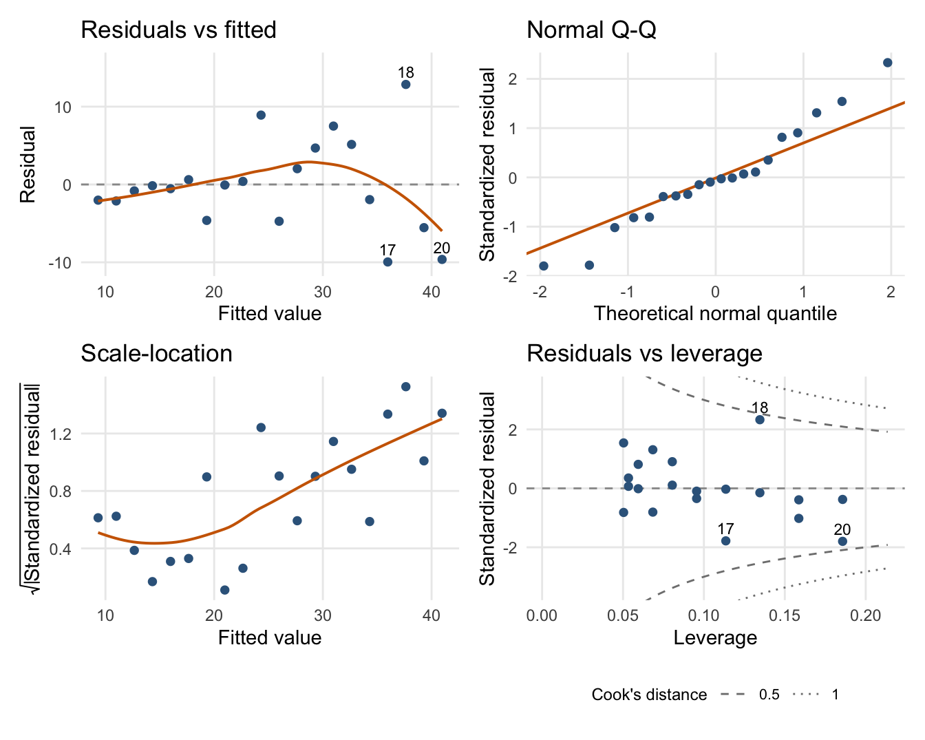
The helper below uses ggplot2 for the plots and patchwork to arrange them. Install patchwork once with install.packages("patchwork") if needed. It draws residuals versus fitted values, a normal Q-Q plot, a scale-location plot, and standardized residuals versus leverage. The last panel includes Cook’s-distance contours; labels identify the three observations with the largest Cook’s distances. For weighted least squares, the first panel uses residuals multiplied by the square root of their weights. The other panels use standardized residuals computed for the fitted model.

lm_diagnostics <- function(fit) {
  stopifnot(inherits(fit, "lm"), !inherits(fit, "glm"))
  d <- data.frame(fitted = fitted(fit),
                  residual = weighted.residuals(fit),
                  standardized = rstandard(fit),
                  leverage = hatvalues(fit),
                  cooks_distance = cooks.distance(fit))
  d$observation <- rownames(d)
  d$scale_location <- sqrt(abs(d$standardized))
  marked <- d[head(order(d$cooks_distance, decreasing = TRUE), 3), ]

  residual_plot <- ggplot(d, aes(fitted, residual)) +
    geom_hline(yintercept = 0, linetype = "dashed", colour = "grey60") +
    geom_point(colour = "steelblue4", size = 1.7) +
    geom_smooth(method = "loess", formula = y ~ x, span = 1,
                 se = FALSE, colour = "darkorange3", linewidth = 0.7) +
    geom_text(data = marked, aes(label = observation), vjust = -0.6,
               size = 3, check_overlap = TRUE) +
    scale_y_continuous(expand = expansion(mult = c(0.08, 0.18))) +
    labs(title = "Residuals vs fitted", x = "Fitted value",
         y = if (is.null(weights(fit))) "Residual" else "Weighted residual")

  qq_plot <- ggplot(d, aes(sample = standardized)) +
    stat_qq_line(colour = "darkorange3", linewidth = 0.7) +
    stat_qq(colour = "steelblue4", size = 1.7) +
    labs(title = "Normal Q-Q", x = "Theoretical normal quantile",
         y = "Standardized residual")

  scale_plot <- ggplot(d, aes(fitted, scale_location)) +
    geom_point(colour = "steelblue4", size = 1.7) +
    geom_smooth(method = "loess", formula = y ~ x, span = 1,
                 se = FALSE, colour = "darkorange3", linewidth = 0.7) +
    labs(title = "Scale-location", x = "Fitted value",
         y = expression(sqrt(abs("Standardized residual"))))

  contours <- expand.grid(
    leverage = seq(0.001, min(0.99, max(d$leverage) * 1.15),
      length.out = 200),
    distance = c(0.5, 1), sign = c(-1, 1))
  contours$standardized <- with(contours,
    sign * sqrt(distance * fit$rank * (1 - leverage) / leverage))
  limit <- max(3, abs(d$standardized)) * 1.15
  leverage_plot <- ggplot(d, aes(leverage, standardized)) +
    geom_hline(yintercept = 0, linetype = "dashed", colour = "grey60") +
    geom_line(data = contours,
               aes(group = interaction(distance, sign),
                 linetype = factor(distance)),
               colour = "grey50", linewidth = 0.5) +
    geom_point(colour = "steelblue4", size = 1.7) +
    geom_text(data = marked, aes(label = observation), vjust = -0.6,
               size = 3, check_overlap = TRUE) +
    scale_linetype_manual(values = c("dashed", "dotted")) +
    coord_cartesian(ylim = c(-limit, limit)) +
    labs(title = "Residuals vs leverage", x = "Leverage",
         y = "Standardized residual", linetype = "Cook's distance") +
    theme(legend.text = element_text(size = 8),
          legend.title = element_text(size = 9))

  patchwork::wrap_plots(residual_plot, qq_plot, scale_plot, leverage_plot,
    ncol = 2)
}

lm_diagnostics(fit)

Figure 8.2: Diagnostic plots for the eight-observation example. The observation labels identify large Cook’s distances.

Extract basic diagnostics numerically

data.frame(
  fitted = fitted(fit),
  residual = resid(fit),
  std_resid = rstandard(fit),
  stud_resid = rstudent(fit),
  leverage = hatvalues(fit),
  cooks_d = cooks.distance(fit)
)

      fitted   residual  std_resid stud_resid  leverage     cooks_d
1  0.3333333  1.6666667  0.6930976  0.6596673 0.4166667 0.171565824
2  3.0238095  0.9761905  0.3638424  0.3358671 0.2738095 0.024957133
3  5.7142857 -0.7142857 -0.2503174 -0.2297101 0.1785714 0.006810742
4  8.4047619 -0.4047619 -0.1379056 -0.1260900 0.1309524 0.001432860
5 11.0952381 -1.0952381 -0.3731563 -0.3446665 0.1309524 0.010491110
6 13.7857143 -2.7857143 -0.9762380 -0.9716857 0.1785714 0.103591380
7 16.4761905 -3.4761905 -1.2956340 -1.3936654 0.2738095 0.316470107
8 19.1666667  5.8333333  2.4258417 15.9752413 0.4166667 2.101681345

Identify potentially unusual observations

which(abs(rstudent(fit)) > 2)

8
8 

which(hatvalues(fit) > 2 * length(coef(fit)) / nrow(dat))

named integer(0)

which(cooks.distance(fit) > 4 / nrow(dat))

8
8 

Example With Heteroscedasticity-Like Pattern

set.seed(8561)
x2 <- seq(1, 20, by = 1)
y2 <- 5 + 2 * x2 + rnorm(length(x2), sd = x2 / 3)

dat2 <- data.frame(x = x2, y = y2)
fit2 <- lm(y ~ x, data = dat2)

lm_diagnostics(fit2)

Figure 8.3: Diagnostics for simulated errors whose variance increases with x.

Example With Curvature

set.seed(8561)
x3 <- seq(-3, 3, length.out = 40)
y3 <- 2 + x3 + 1.5 * x3^2 + rnorm(length(x3), sd = 1)

dat3 <- data.frame(x = x3, y = y3)
fit3 <- lm(y ~ x, data = dat3)

lm_diagnostics(fit3)

Figure 8.4: Diagnostics when a straight-line mean is fitted to data with curvature.

Comparing a Linear and Quadratic Fit

fit3_quad <- lm(y ~ x + I(x^2), data = dat3)
anova(fit3, fit3_quad)

Analysis of Variance Table

Model 1: y ~ x
Model 2: y ~ x + I(x^2)
  Res.Df    RSS Df Sum of Sq      F    Pr(>F)
1     38 803.70
2     37  58.49  1    745.22 471.45 < 2.2e-16 ***
---
Signif. codes:  0 '***' 0.001 '**' 0.01 '*' 0.05 '.' 0.1 ' ' 1

summary(fit3_quad)

Call:
lm(formula = y ~ x + I(x^2), data = dat3)

Residuals:
     Min       1Q   Median       3Q      Max
-2.66753 -0.78482  0.07729  0.64825  2.42384

Coefficients:
            Estimate Std. Error t value Pr(>|t|)
(Intercept)  1.91995    0.29834   6.435 1.62e-07 ***
x            0.91401    0.11194   8.165 8.45e-10 ***
I(x^2)       1.53156    0.07054  21.713  < 2e-16 ***
---
Signif. codes:  0 '***' 0.001 '**' 0.01 '*' 0.05 '.' 0.1 ' ' 1

Residual standard error: 1.257 on 37 degrees of freedom
Multiple R-squared:  0.9357,    Adjusted R-squared:  0.9322
F-statistic: 269.1 on 2 and 37 DF,  p-value: < 2.2e-16

Interpreting Software Output

In practice, useful commands in R include:

• lm_diagnostics(fit) for the standard diagnostic panel;
• resid(fit) for residuals;
• rstandard(fit) for standardized residuals;
• rstudent(fit) for studentized residuals;
• hatvalues(fit) for leverages;
• cooks.distance(fit) for Cook’s distances.

Students should learn to connect each numerical output to a concrete modelling question.

A Practical Diagnostic Workflow

A sensible basic workflow is:

• inspect the scatterplot and fitted line;
• examine the residuals-versus-fitted plot;
• check the normal Q-Q plot;
• inspect leverage and Cook’s distance;
• investigate any unusual observations directly in the data;
• decide whether model revision is needed.

This sequence often works well for both simple and multiple regression.

What To Do After Finding a Problem

Finding a diagnostic issue does not mean we automatically delete observations. Instead, possible next steps include:

• checking for data entry or measurement errors;
• understanding whether the point represents a different regime;
• refitting with and without the point for sensitivity analysis;
• revising the model form;
• transforming variables;
• reporting the issue transparently.

Model criticism should be thoughtful, not mechanical.

In-Class Discussion Questions

1. Why are raw residuals not enough for identifying unusual observations?
2. Why can a high-leverage point have a small residual and still matter?
3. Why is Cook’s distance more about influence than outlyingness?
4. What kinds of model failure are easiest to detect from a residual-versus-fitted plot?

8.5 Practice Problems

Conceptual

1. Explain the difference between an outlier, a high-leverage observation, and an influential observation.
2. Explain why residuals have unequal variance.
3. Explain why a normal Q-Q plot is useful even though residuals are not independent.

Computational

Suppose a regression model has \(n=25\) observations and \(p=4\) parameters.

1. Compute the rough leverage benchmark \(2p/n\).
2. If one observation has \(h_{ii}=0.45\), explain whether this seems unusually large.
3. Suppose an observation has a large studentized residual but very small leverage. What kind of problem does this suggest?
4. Suppose another observation has large leverage but a very small residual. Why might it still deserve attention?

Model-Criticism Problem

A residual-versus-fitted plot shows a clear U-shape.

1. What model assumption is likely failing?
2. What changes to the model might you consider?
3. Why would simply reporting coefficient \(p\)-values be insufficient here?

Suggested Take home exercise

Complete the following tasks:

• fit a regression model in R and produce the standard diagnostic plots;
• identify any observations with large studentized residuals, high leverage, or large Cook’s distance;
• write a short interpretation of each diagnostic plot;
• modify a model to address one detected issue, such as curvature or unequal variance;
• compare the original and revised models.

Summary

In this chapter, we studied model diagnostics for linear regression. We focused on:

• residuals and standardized residuals;
• fitted-versus-residual plots;
• normal Q-Q plots;
• leverage and influence;
• Cook’s distance and related ideas;
• practical judgment in assessing model adequacy.

These ideas are essential because regression analysis is not complete until the fitted model has been critically examined.