A useful model must answer a stated question. Estimating an adjusted association, comparing treatments, and predicting a future response can favor different choices. This chapter keeps the main principles of collinearity and validation; automatic selection algorithms are in an optional appendix.
10.1 Stable estimates and scientific questions
Collinearity. When columns of \(X\) are nearly dependent, different coefficient combinations can produce very similar fitted values. The covariance \(\sigma^2(X^\top X)^{-1}\) then explains why individual coefficients can be unstable even when fitted values are reasonably precise.
For a single nonconstant predictor column, \(\operatorname{VIF}_j=1/(1-R_j^2)\), where \(R_j^2\) comes from regressing that column on the other predictors with an intercept. A large value is a diagnostic clue, not an automatic rule for deleting variables. Multi-column factors require additional care in interpreting column-specific VIFs.
Keep the question fixed. Removing a covariate changes the adjusted comparison. Retain terms required by the scientific question or design, and respect hierarchy when including interactions. Centering can clarify an intercept or reduce some polynomial-column correlations, but it does not create new information.
ImportantSelection changes inference
Intervals and tests derived for a prespecified model do not automatically retain their interpretation after searching the data for a favorable model. A training/test split or cross-validation estimates predictive performance; it does not by itself validate post-selection coefficient intervals.
10.2 Comparing predictive performance
Training SSE and training \(R^2\) reward added flexibility. Predictive evaluation instead asks how a fitted procedure behaves on observations it did not use for fitting.
A simple workflow. Specify a small set of candidate models, use the same observations and the same folds, fit each model only on the training portion, and evaluate it on the held-out portion. Any imputation, centering, feature construction, or variable search learned from data belongs inside the training step. If validation is used to choose a model, its winning validation error is itself optimistic; use an untouched test set or nested resampling for a final performance claim.
For continuous responses, one useful loss is \(\operatorname{MSE}_{test}=m^{-1}\sum_{i=1}^m(y_i-\hat y_i)^2\). For binary and count outcomes, the GLM chapter introduces response-appropriate interpretation and predictive checks.
NoteRespect the observational unit
Random row-wise folds are appropriate only when they match the intended prediction setting. With repeated measurements, keep a subject’s observations together; with temporal prediction, evaluate on later periods. A large number of rows is not a substitute for independent subjects or future time periods.
AIC and model comparison. AIC balances likelihood fit and parameter count. It is useful when candidate likelihoods refer to the same response and comparable data, but it is not an effect estimate or a significance test. Comparing AIC values from a model for \(Y\) and one for \(\log Y\) requires accounting for the transformation of the likelihood; do not compare the raw software values mechanically. BIC, \(C_p\), and automatic searches are in Automatic Model Selection (Optional).
10.3 A small validation example
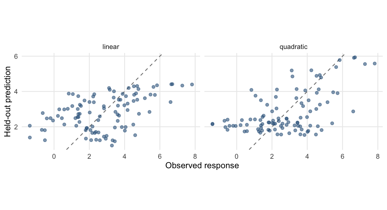
The following simulated curvature example uses the same five folds for two prespecified mean models. It illustrates predictive evaluation, not a guarantee that a quadratic model will always win.
Show R code
library(ggplot2)theme_set(theme_minimal(base_size =11) +theme(legend.position ="bottom",panel.grid.minor =element_blank()))set.seed(8561)n <-100x <-runif(n, -2, 2)dat <-data.frame(x = x, y =2+ x +0.7* x^2+rnorm(n, sd =1.5))fold <-sample(rep(1:5, length.out = n))models <-list(linear = y ~ x, quadratic = y ~ x +I(x^2))pred <-matrix(NA_real_, n, length(models),dimnames =list(NULL, names(models)))for (k in1:5) {for (j inseq_along(models)) { fit <-lm(models[[j]], data = dat[fold != k, ]) pred[fold == k, j] <-predict(fit, newdata = dat[fold == k, ]) }}cv_mse <-colMeans((dat$y - pred)^2)cv_mse
Figure 10.1: Predictions made for held-out observations. Every plotted prediction comes from a fit that excluded that observation’s fold.
Report more than a winner. State the loss, the splitting rule, the population or future setting of interest, and how much performance differs. Investigate poor predictions. A single difference in estimated MSE does not establish a universal ranking of the methods.
10.4 Practice
Explain why adding a predictor can improve training fit without improving held-out predictions.
Explain why a confounder or design variable should not be removed solely because of its p-value or VIF.
Adapt the example to grouped data by assigning folds at the group level.
Write a short report distinguishing an inferential conclusion about a coefficient from a predictive conclusion about a fitted procedure.