Generalized Least Squares and Correlated Errors (Optional)

In this optional topic, we study what happens when the error terms in a linear model are no longer independent with common variance. This leads to generalized least squares, a natural extension of ordinary least squares that accounts for nonidentity covariance structure. The goal is to help students understand how the linear model changes when observations are correlated or have unequal precision in a more general matrix form.

NoteOptional topic: GLS is different from GLM

GLS retains the mean model \(\mathbb{E}(Y)=X\beta\) and changes the error covariance. A generalized linear model instead specifies a response family and a link for its conditional mean. This topic is supplementary to the main course.

Learning Objectives

By the end of this chapter, students should be able to:

• explain why ordinary least squares is not always appropriate when errors are correlated or heteroscedastic;
• state the generalized least squares covariance assumption for the error vector in a linear model context;
• derive the generalized least squares estimator;
• explain how generalized least squares reduces to ordinary least squares and weighted least squares in special cases;
• interpret the transformed-model view of generalized least squares;
• recognize practical examples of correlated errors and structured covariance models.

Reading

Recommended reading for this chapter:

• Seber and Lee:
  • sections on generalized least squares
  • correlated observations and covariance structure
  • extensions of least squares methods
• Montgomery, Peck, and Vining:
  • sections on departures from ordinary linear model assumptions
  • weighted and generalized least squares ideas
  • practical modelling considerations for dependence and unequal variance

Why Ordinary Least Squares Can Fail

So far, much of the course has relied on the classical assumption

\[ \mathrm{Var}(\boldsymbol{\varepsilon}) = \sigma^2 \mathbf{I}_n. \]

This means:

• all observations have the same error variance;
• errors are uncorrelated.

But many real datasets do not satisfy this assumption. Examples include:

• repeated observations on the same unit;
• measurements taken over time;
• clustered or grouped data;
• observations with known unequal precision;
• spatial or serial dependence.

In such cases, ordinary least squares may still be unbiased for the mean model under suitable assumptions, but it is not generally the most efficient linear unbiased estimator, and its usual spherical-error standard errors need not be valid. Unbiasedness still requires a correctly specified conditional mean.

Review of the Linear Model

Recall the linear model

\[ \mathbf{Y} = \mathbf{X}\boldsymbol{\beta} + \boldsymbol{\varepsilon}, \]

with

\[ \mathbb{E}[\boldsymbol{\varepsilon}] = \mathbf{0}. \]

Under ordinary least squares, we assumed

\[ \mathrm{Var}(\boldsymbol{\varepsilon}) = \sigma^2 \mathbf{I}_n. \]

This gave the estimator

\[ \hat{\boldsymbol{\beta}}_{OLS} = (\mathbf{X}^\top \mathbf{X})^{-1}\mathbf{X}^\top \mathbf{Y}. \]

Now we allow a more general covariance structure.

A More General Covariance Model

Suppose instead that

\[ \mathrm{Var}(\boldsymbol{\varepsilon}) = \sigma^2 \mathbf{V}, \]

where \(\mathbf{V}\) is a known positive definite matrix. Then

\[ \mathrm{Var}(\mathbf{Y}) = \sigma^2 \mathbf{V}. \]

The matrix \(\mathbf{V}\) may represent:

• unequal variances;
• correlations among observations;
• both at once.

This is the setting of generalized least squares.

Why the Covariance Matrix Matters

The effect of correlation depends on the quantity being estimated. For equal marginal variance \(\sigma^2\) and correlation \(\rho\), \(\operatorname{Var}\{(Y_1+Y_2)/2\}=\sigma^2(1+\rho)/2\), whereas \(\operatorname{Var}(Y_1-Y_2)=2\sigma^2(1-\rho)\). Positive correlation increases uncertainty for the pair average but decreases it for the within-pair difference. If one observation has much larger variance than another, it should typically receive less weight in estimation.

Thus the covariance structure affects how much information each part of the data contributes. Ordinary least squares ignores this structure. Generalized least squares incorporates it directly.

The Generalized Least Squares Criterion

In generalized least squares, we minimize the quadratic form

\[ Q(\boldsymbol{\beta}) = (\mathbf{Y} - \mathbf{X}\boldsymbol{\beta})^\top \mathbf{V}^{-1} (\mathbf{Y} - \mathbf{X}\boldsymbol{\beta}). \]

This is the natural analogue of the ordinary least squares criterion

\[ (\mathbf{Y} - \mathbf{X}\boldsymbol{\beta})^\top (\mathbf{Y} - \mathbf{X}\boldsymbol{\beta}), \]

but now weighted by the inverse covariance structure. The matrix \(\mathbf{V}^{-1}\) downweights directions in the data that are more variable or more redundant.

Derivation of the Generalized Least Squares Estimator

Differentiate the generalized least squares criterion with respect to \(\boldsymbol{\beta}\) and set the derivative equal to zero. This gives the generalized normal equations

\[ \mathbf{X}^\top \mathbf{V}^{-1}\mathbf{X}\,\hat{\boldsymbol{\beta}}_{GLS} = \mathbf{X}^\top \mathbf{V}^{-1}\mathbf{Y}. \]

Assuming invertibility, the generalized least squares estimator is

\[ \hat{\boldsymbol{\beta}}_{GLS} = (\mathbf{X}^\top \mathbf{V}^{-1}\mathbf{X})^{-1} \mathbf{X}^\top \mathbf{V}^{-1}\mathbf{Y}. \]

This is the central formula for the week.

Interpretation of the GLS Estimator

The GLS estimator has the same structural form as OLS and WLS, but with the covariance matrix inserted. It can be interpreted as an estimator that gives appropriate weight to observations according to the joint covariance structure. Compared with OLS:

• observations with larger variance are effectively downweighted;
• correlated observations are not treated as if they were independent;
• the estimator uses the information in the data more efficiently when \(\mathbf{V}\) is correctly specified.

Special Case: Ordinary Least Squares

If \(\mathbf{V} = \mathbf{I}_n\), then GLS becomes

\[ \hat{\boldsymbol{\beta}}_{GLS} = (\mathbf{X}^\top \mathbf{X})^{-1}\mathbf{X}^\top \mathbf{Y}, \]

which is exactly the ordinary least squares estimator. So OLS is a special case of GLS.

Special Case: Weighted Least Squares

If the covariance matrix is diagonal, \(\mathbf{V} = \mathrm{diag}(v_1,\dots,v_n)\), then

\[ \mathbf{V}^{-1} = \mathrm{diag}(1/v_1,\dots,1/v_n). \]

This is the weighted least squares setting from Chapter 9 — Transformations and Weighted Least Squares, with weights proportional to inverse variances. So WLS is also a special case of GLS.

The Transformed-Model View

A very important way to understand GLS is through a transformation. Because \(\mathbf{V}\) is positive definite, there exists a matrix \(\mathbf{A}\) such that

\[ \mathbf{A}^\top \mathbf{A} = \mathbf{V}^{-1}. \]

For example, we may take \(\mathbf{A} = \mathbf{V}^{-1/2}\). Multiplying the model by \(\mathbf{A}\) gives

\[ \mathbf{A}\mathbf{Y} = \mathbf{A}\mathbf{X}\boldsymbol{\beta} + \mathbf{A}\boldsymbol{\varepsilon}. \]

Now the transformed error has variance

\[ \mathrm{Var}(\mathbf{A}\boldsymbol{\varepsilon}) = \mathbf{A}(\sigma^2 \mathbf{V})\mathbf{A}^\top = \sigma^2 \mathbf{I}_n. \]

So GLS can be viewed as ordinary least squares applied to a transformed model with spherical errors. This is one of the most important conceptual ideas in the course.

Distribution of the GLS Estimator

If the covariance structure is correctly specified and

\[ \mathbf{Y} \sim N_n(\mathbf{X}\boldsymbol{\beta}, \sigma^2 \mathbf{V}), \]

then the GLS estimator is normally distributed:

\[ \hat{\boldsymbol{\beta}}_{GLS} \sim N_p\!\left( \boldsymbol{\beta}, \sigma^2 (\mathbf{X}^\top \mathbf{V}^{-1}\mathbf{X})^{-1} \right). \]

This parallels the OLS distribution theory, but with \(\mathbf{V}^{-1}\) appearing throughout.

Gauss-Markov Interpretation

Under the covariance model

\[ \mathrm{Var}(\boldsymbol{\varepsilon}) = \sigma^2 \mathbf{V}, \]

the generalized least squares estimator is the best linear unbiased estimator among all linear unbiased estimators. So GLS is the natural Gauss-Markov extension of OLS to nonidentity covariance structures. This is sometimes phrased by saying that OLS is BLUE under spherical errors, while GLS is BLUE under the more general covariance model.

Estimating Sigma Squared Under GLS

In the transformed model, residual sums of squares can be defined using the GLS criterion. The generalized residual sum of squares is

\[ SSE_{GLS} = (\mathbf{Y} - \mathbf{X}\hat{\boldsymbol{\beta}}_{GLS})^\top \mathbf{V}^{-1} (\mathbf{Y} - \mathbf{X}\hat{\boldsymbol{\beta}}_{GLS}). \]

Under the normal model with known \(\mathbf{V}\), this plays the same role as the ordinary SSE after transformation. An estimator of \(\sigma^2\) is then

\[ \hat{\sigma}^2_{GLS} = \frac{SSE_{GLS}}{n-p}. \]

Why Known V Is Rare

In practice, the covariance matrix \(\mathbf{V}\) is usually not known exactly. Instead, we may have:

• scientific knowledge suggesting a covariance pattern;
• repeated-measures structure suggesting dependence;
• known weights from design considerations;
• an estimated covariance model.

When \(\mathbf{V}\) is replaced by an estimate, the resulting estimator is often called feasible GLS.

Feasible Weighted Least Squares

In many applications, the variances are not known exactly. Instead, we estimate the variance pattern from the data and then use estimated weights. This is often called feasible weighted least squares. Typical workflow:

• fit an initial OLS model;
• inspect residuals to understand how variance changes;
• propose a variance model;
• compute estimated weights;
• refit using WLS.

This approach is practical, though it introduces additional modelling decisions.

ImportantKnown versus estimated covariance

Exact normal-model t and F distributions apply to the transformed model when the relative covariance is known and the remaining assumptions hold. Plugging in estimated weights or covariance parameters does not automatically preserve those exact distributions.

Feasible Generalized Least Squares

The basic idea of feasible GLS is:

• propose a covariance model for \(\mathbf{V}\);
• estimate the unknown covariance parameters from the data;
• plug the estimated covariance matrix into the GLS formula.

This is practical, but it introduces an extra modelling step and relies on the covariance model being approximately correct.

Examples of Covariance Structures

Several structured covariance matrices appear often in applications.

Unequal Variances Only

If observations are independent but have different variances, then \(\mathbf{V}\) is diagonal. This is the weighted least squares case.

Compound Symmetry

In grouped or repeated-measures settings, one may assume a common variance and a common correlation within group. This gives a covariance pattern often called compound symmetry.

Autoregressive Structure

For time-ordered observations, nearby errors may be more strongly correlated than distant ones. A simple model is the AR(1) structure, where correlations decay geometrically with lag.

Block-Diagonal Structure

If observations are grouped into independent clusters, then \(\mathbf{V}\) may be block diagonal, with each block describing within-cluster dependence. These examples help students see that covariance structure is part of model formulation, not just a technical afterthought.

Correlated Errors in Time-Ordered Data

Suppose we observe data over time:

\[ Y_t = \beta_0 + \beta_1 x_t + \varepsilon_t. \]

If the errors satisfy

\[ \mathrm{Corr}(\varepsilon_t,\varepsilon_{t-1}) \neq 0, \]

then ordinary least squares may still estimate the mean trend, but standard errors based on independence are not trustworthy. This is one of the classic motivations for generalized least squares.

Clustered and Repeated Observations

Suppose several observations come from the same individual, school, hospital, or geographic region. Then responses within the same cluster may be correlated. In this case, the assumption of independent errors is not appropriate, and a structured covariance model or a mixed-model approach may be better suited. GLS provides an important stepping stone toward these more advanced frameworks.

Relationship to Robust Standard Errors

One alternative to full covariance modelling is to keep the OLS mean estimator but adjust the standard errors to be robust to heteroscedasticity or dependence. This is a different strategy from GLS.

• GLS changes the estimator itself using a covariance model;
• robust standard errors keep the estimator but correct inference approximately.

Both are useful, but they serve different purposes. This distinction is valuable for students to understand even if robust methods are treated only briefly.

When GLS Is Worth Using

GLS is especially attractive when:

• there is a defensible covariance model;
• the dependence or heteroscedasticity is substantial;
• efficient estimation matters;
• the transformed model remains interpretable.

If the covariance model is poorly specified, the gains from GLS may be limited, and robustness or alternative modelling strategies may be preferable.

Diagnostics for Correlated Errors

Symptoms that may suggest correlated errors include:

• residuals that display runs or systematic temporal patterns;
• residual plots against time showing clustering;
• repeated-measures structure built into the design;
• known grouping or spatial dependence in the data collection process.

The key lesson is that covariance structure should be motivated both by diagnostics and by how the data were collected.

Worked Example With Known Unequal Precision

Suppose each response is an average of \(m_i\) repeated measurements. Then the variance of the average may satisfy

\[ \mathrm{Var}(Y_i) = \frac{\sigma^2}{m_i}. \]

In that case, a natural choice is

\[ v_i = \frac{1}{m_i}, \qquad w_i = m_i. \]

So observations based on more repeated measurements get more weight. This is a very intuitive example of GLS through weighted least squares.

Worked Example With Correlated Pairs

Suppose observations come in natural pairs, and within each pair the errors are positively correlated. Then the covariance matrix has a block structure, with a \(2\times2\) covariance block for each pair. GLS accounts for covariance when estimating the target mean or contrast. For positive within-pair correlation, averaging and differencing have different information consequences; compare their variances above.

R Demonstration With Weighted Least Squares as GLS

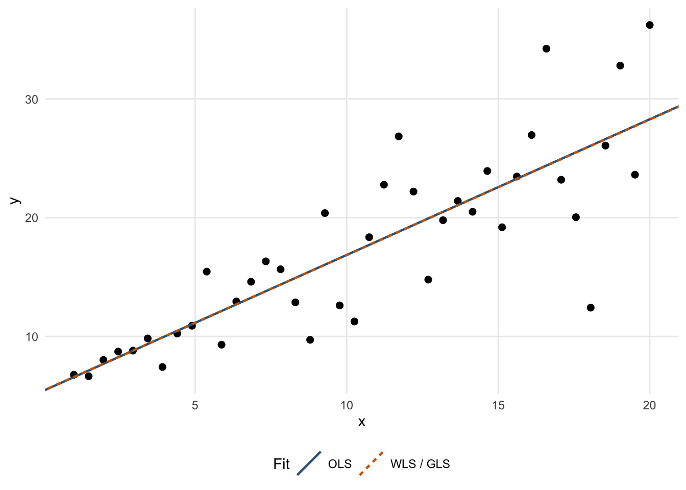
Simulate data with unequal variances

library(ggplot2)
theme_set(theme_minimal(base_size = 11) +
            theme(legend.position = "bottom",
              panel.grid.minor = element_blank()))

set.seed(8561)
n <- 40
x <- seq(1, 20, length.out = n)
v <- 0.3 + 0.08 * x^2
y <- 5 + 1.2 * x + rnorm(n, sd = sqrt(v))

dat <- data.frame(y = y, x = x, v = v)

fit_ols <- lm(y ~ x, data = dat)
fit_wls <- lm(y ~ x, data = dat, weights = 1 / v)

summary(fit_ols)

Call:
lm(formula = y ~ x, data = dat)

Residuals:
    Min      1Q  Median      3Q     Max
-13.636  -2.163   0.190   1.948   9.834

Coefficients:
            Estimate Std. Error t value Pr(>|t|)
(Intercept)   5.4316     1.4586   3.724 0.000635 ***
x             1.1426     0.1225   9.331 2.26e-11 ***
---
Signif. codes:  0 '***' 0.001 '**' 0.01 '*' 0.05 '.' 0.1 ' ' 1

Residual standard error: 4.356 on 38 degrees of freedom
Multiple R-squared:  0.6962,    Adjusted R-squared:  0.6882
F-statistic: 87.07 on 1 and 38 DF,  p-value: 2.257e-11

summary(fit_wls)

Call:
lm(formula = y ~ x, data = dat, weights = 1/v)

Weighted Residuals:
     Min       1Q   Median       3Q      Max
-2.65080 -0.75591  0.07032  0.67369  2.38994

Coefficients:
            Estimate Std. Error t value Pr(>|t|)
(Intercept)  5.44884    0.47201   11.54 5.46e-14 ***
x            1.14032    0.08545   13.34 6.42e-16 ***
---
Signif. codes:  0 '***' 0.001 '**' 0.01 '*' 0.05 '.' 0.1 ' ' 1

Residual standard error: 1.239 on 38 degrees of freedom
Multiple R-squared:  0.8241,    Adjusted R-squared:  0.8195
F-statistic: 178.1 on 1 and 38 DF,  p-value: 6.418e-16

Compare fitted lines

line_fits <- data.frame(model = c("OLS", "WLS / GLS"),
                        intercept = c(coef(fit_ols)[1], coef(fit_wls)[1]),
                        slope = c(coef(fit_ols)[2], coef(fit_wls)[2]))
ggplot(dat, aes(x, y)) +
  geom_point(size = 2) +
  geom_abline(data = line_fits,
              aes(intercept = intercept, slope = slope, colour = model,
                linetype = model),
              linewidth = 0.8) +
  scale_colour_manual(values = c("OLS" = "steelblue4",
    "WLS / GLS" = "darkorange3")) +
  labs(x = "x", y = "y", colour = "Fit", linetype = "Fit")

Figure 1: OLS and WLS fitted lines when the relative observation variances are known.

R Demonstration With a Hand-Built GLS Computation

Construct a covariance matrix and compute GLS directly

set.seed(8561)
n2 <- 8
x2 <- seq(1, n2)
X <- cbind(1, x2)

rho <- 0.6
V <- outer(1:n2, 1:n2, function(i, j) rho^abs(i - j))
beta_true <- c(2, 1.5)

eps <- t(chol(V)) %*% rnorm(n2)
y2 <- as.vector(X %*% beta_true + eps)

Y <- matrix(y2, ncol = 1)

beta_gls <- solve(t(X) %*% solve(V) %*% X) %*% t(X) %*% solve(V) %*% Y
beta_ols <- solve(t(X) %*% X) %*% t(X) %*% Y

beta_gls

       [,1]
   3.336799
x2 1.299329

beta_ols

       [,1]
   3.379372
x2 1.309102

Transform the model and verify the GLS view

A <- solve(t(chol(V))) # chol(V) is upper triangular: V = R'R
Y_tilde <- A %*% Y
X_tilde <- A %*% X

beta_transformed <- solve(t(X_tilde) %*% X_tilde) %*% t(X_tilde) %*% Y_tilde
beta_transformed

       [,1]
   3.336799
x2 1.299329

max(abs(beta_transformed - beta_gls)) # numerical agreement with direct GLS

[1] 9.769963e-15

max(abs(A %*% V %*% t(A) - diag(n2))) # whitening check

[1] 1.804112e-16

Compare residual patterns

fit_ols2 <- lm(y2 ~ x2)
ordered_residuals <- data.frame(time = x2, residual = resid(fit_ols2))
ggplot(ordered_residuals, aes(time, residual)) +
  geom_hline(yintercept = 0, linetype = "dashed", colour = "grey50") +
  geom_line(colour = "steelblue4", linewidth = 0.7) +
  geom_point(colour = "steelblue4", size = 2) +
  labs(x = "Time order", y = "OLS residual")

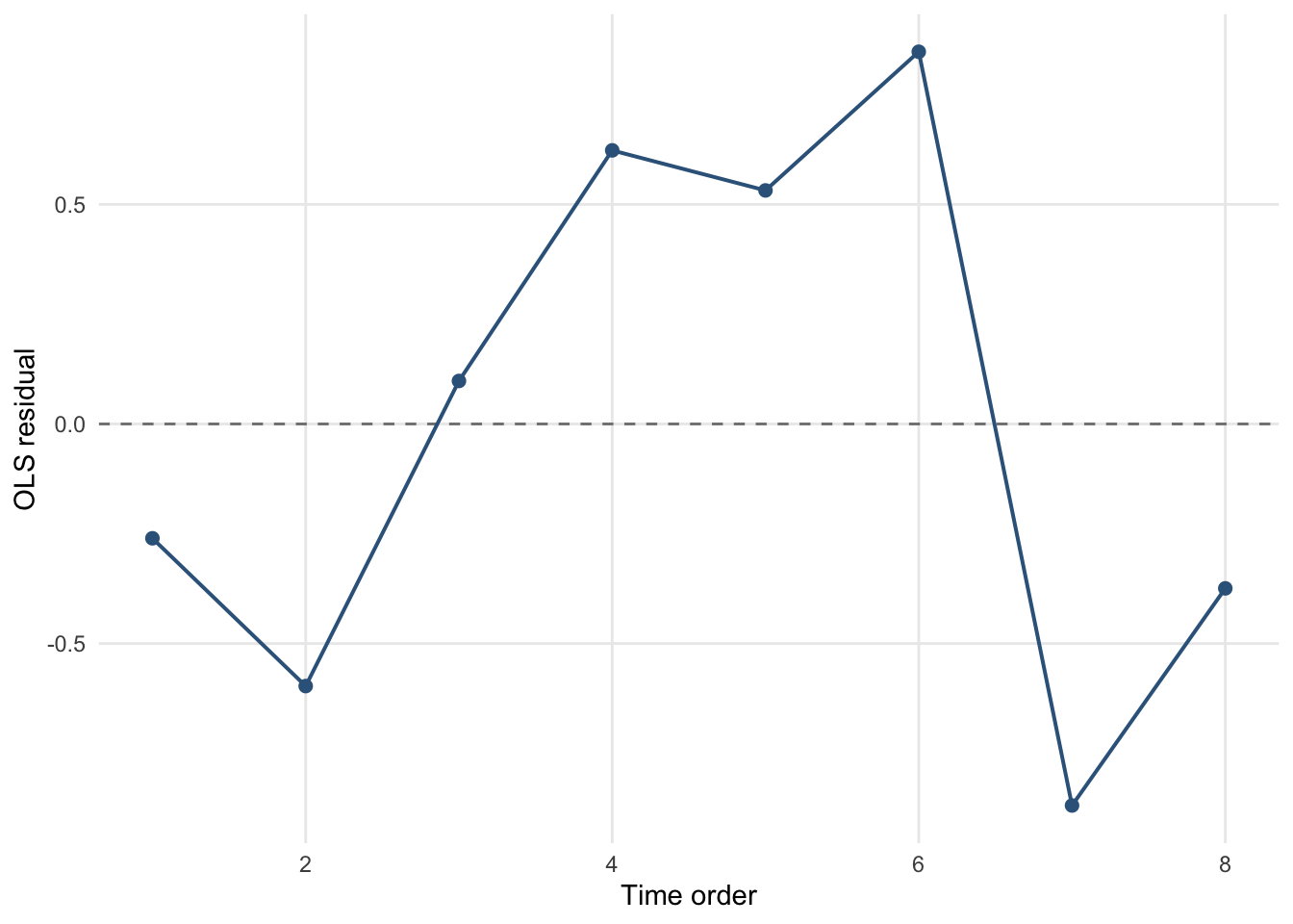
Figure 2: OLS residuals in time order for the simulated correlated-error example.

Simple example of grouped covariance intuition

set.seed(8561)
group <- rep(1:10, each = 3)
x3 <- rnorm(length(group))
u <- rnorm(10, sd = 1.2)
eps3 <- rep(u, each = 3) + rnorm(length(group), sd = 0.5)
y3 <- 4 + 2 * x3 + eps3

dat3 <- data.frame(y = y3, x = x3, group = factor(group))
fit3 <- lm(y ~ x, data = dat3)
summary(fit3)

Call:
lm(formula = y ~ x, data = dat3)

Residuals:
    Min      1Q  Median      3Q     Max
-3.3937 -0.8770 -0.0909  0.9381  2.9870

Coefficients:
            Estimate Std. Error t value Pr(>|t|)
(Intercept)   3.7464     0.2929  12.789 3.27e-13 ***
x             2.1451     0.2450   8.757 1.66e-09 ***
---
Signif. codes:  0 '***' 0.001 '**' 0.01 '*' 0.05 '.' 0.1 ' ' 1

Residual standard error: 1.603 on 28 degrees of freedom
Multiple R-squared:  0.7325,    Adjusted R-squared:  0.723
F-statistic: 76.68 on 1 and 28 DF,  p-value: 1.656e-09

Interpreting Software Output

In base R, ordinary lm() directly handles OLS and weighted least squares through the weights= argument. More general correlated-error models often require additional packages in practice, but the matrix formula is already enough to understand the core idea of GLS. Students should focus on:

• what covariance structure is being assumed;
• why that structure is plausible;
• how the weighting or transformation changes the estimator;
• what practical goal is being improved.

A Practical Workflow for GLS Thinking

A sensible workflow is:

• ask whether independence and equal variance are plausible from the design of the study;
• inspect residual patterns for signs of heteroscedasticity or dependence;
• propose a covariance structure or weighting scheme when justified;
• compare OLS and GLS-style fits;
• interpret the results in light of both efficiency and model credibility.

In-Class Discussion Questions

1. Why is weighted least squares a special case of generalized least squares?
2. Why can correlated observations carry less information than independent observations?
3. What is the conceptual benefit of the transformed-model view of GLS?
4. When might robust standard errors be preferred to specifying a full covariance model?

Practice Problems

Conceptual

1. Explain why OLS is not generally efficient when the covariance matrix is not proportional to the identity.
2. Explain how GLS uses the inverse covariance matrix to weight information in the data.
3. Explain the difference between modelling the covariance structure and simply correcting standard errors.

Computational

Suppose

\[ \mathrm{Var}(\boldsymbol{\varepsilon}) = \sigma^2 \mathbf{V}, \qquad \mathbf{V} = \begin{pmatrix} 1 & 0 \\ 0 & 4 \end{pmatrix}. \]

1. Write down \(\mathbf{V}^{-1}\).
2. Which observation receives more weight in GLS?
3. Explain why.

Now suppose

\[ \hat{\boldsymbol{\beta}}_{GLS} = (\mathbf{X}^\top \mathbf{V}^{-1}\mathbf{X})^{-1} \mathbf{X}^\top \mathbf{V}^{-1}\mathbf{Y}. \]

1. Show how this reduces to OLS when \(\mathbf{V} = \mathbf{I}_n\).
2. Show how this reduces to WLS when \(\mathbf{V}\) is diagonal.

Modelling Problem

You have repeated observations on each subject over time.

1. Why is the independence assumption questionable?
2. What kinds of covariance structure might be reasonable?
3. Why might GLS be more appropriate than OLS in this setting?

Suggested Take home exercise

Complete the following tasks:

• fit an OLS model and a weighted least squares model for data with unequal variance;
• compare coefficient estimates, standard errors, and residual plots;
• compute a GLS estimator by hand for a small example with a known covariance matrix;
• explain the transformed-model view in your own words;
• write a short discussion of when a covariance model is scientifically credible enough to justify GLS.

Summary

In this chapter, we studied generalized least squares as an extension of ordinary least squares to models with nonidentity covariance structure. We emphasized that:

• OLS assumes spherical errors;
• GLS allows unequal variances and correlated errors;
• WLS is a special case of GLS;
• GLS can be understood as OLS on a transformed model;
• covariance structure is part of model formulation and should be justified by both design and diagnostics.