In this week, we study the core idea behind linear regression: least squares estimation . We derive the ordinary least squares estimator, interpret it geometrically as a projection, and introduce the fitted values, residuals, and the hat matrix.
Learning Objectives
By the end of this week, students should be able to:
define the least squares criterion for a linear model;
derive the normal equations;
obtain the ordinary least squares estimator when the design matrix has full column rank;
interpret least squares as an orthogonal projection;
define the fitted values, residuals, and hat matrix;
explain the orthogonality properties of residuals.
Reading
Recommended reading for this week:
Seber and Lee:
Chapter 3: sections on least squares estimation
Montgomery, Peck, and Vining:
introductory sections on estimation in linear regression
1. Review of the Linear Model
Recall the linear model from Week 1:
\[
\mathbf{Y} = \mathbf{X}\boldsymbol{\beta} + \boldsymbol{\varepsilon},
\]
where
\(\mathbf{Y}\) is an \(n \times 1\) response vector,\(\mathbf{X}\) is an \(n \times p\) design matrix,\(\boldsymbol{\beta}\) is a \(p \times 1\) parameter vector,\(\boldsymbol{\varepsilon}\) is an \(n \times 1\) error vector.
Under the classical setup, we often assume
\[
\mathbb{E}[\boldsymbol{\varepsilon}] = \mathbf{0},
\qquad
\mathrm{Var}(\boldsymbol{\varepsilon}) = \sigma^2 \mathbf{I}_n.
\]
Hence,
\[
\mathbb{E}[\mathbf{Y}] = \mathbf{X}\boldsymbol{\beta},
\qquad
\mathrm{Var}(\mathbf{Y}) = \sigma^2 \mathbf{I}_n.
\]
Our goal is to estimate \(\boldsymbol{\beta}\) from the observed data.
2. The Least Squares Criterion
2.1 Motivation
For any candidate value \(\boldsymbol{\beta}\) , the model predicts
\[
\mathbf{X}\boldsymbol{\beta}.
\]
The discrepancy between the observed response \(\mathbf{Y}\) and the model mean \(\mathbf{X}\boldsymbol{\beta}\) is
\[
\mathbf{Y} - \mathbf{X}\boldsymbol{\beta}.
\]
This vector is called the residual vector for the candidate \(\boldsymbol{\beta}\) .
A natural idea is to choose \(\boldsymbol{\beta}\) so that this discrepancy is as small as possible.
2.2 Residual sum of squares
The least squares criterion is
\[
S(\boldsymbol{\beta})
=
(\mathbf{Y} - \mathbf{X}\boldsymbol{\beta})^\top
(\mathbf{Y} - \mathbf{X}\boldsymbol{\beta}).
\]
Equivalently,
\[
S(\boldsymbol{\beta}) = \|\mathbf{Y} - \mathbf{X}\boldsymbol{\beta}\|^2.
\]
We choose \(\hat{\boldsymbol{\beta}}\) to minimize \(S(\boldsymbol{\beta})\) .
2.3 Expansion of the criterion
Expanding the quadratic form gives
\[
S(\boldsymbol{\beta})
=
\mathbf{Y}^\top \mathbf{Y}
- 2\boldsymbol{\beta}^\top \mathbf{X}^\top \mathbf{Y}
+ \boldsymbol{\beta}^\top \mathbf{X}^\top \mathbf{X}\boldsymbol{\beta}.
\]
This is a quadratic function of \(\boldsymbol{\beta}\) .
3. Derivation of the Normal Equations
To minimize \(S(\boldsymbol{\beta})\) , differentiate with respect to \(\boldsymbol{\beta}\) :
\[
\frac{\partial S(\boldsymbol{\beta})}{\partial \boldsymbol{\beta}}
=
-2\mathbf{X}^\top \mathbf{Y} + 2\mathbf{X}^\top \mathbf{X}\boldsymbol{\beta}.
\]
Setting this equal to zero yields the normal equations :
\[
\mathbf{X}^\top \mathbf{X}\hat{\boldsymbol{\beta}}
=
\mathbf{X}^\top \mathbf{Y}.
\]
These are the equations that define the ordinary least squares estimator.
3.1 Full column rank case
If \(\mathbf{X}\) has full column rank \(p\) , then \(\mathbf{X}^\top \mathbf{X}\) is invertible, and the unique least squares estimator is
\[
\hat{\boldsymbol{\beta}}
=
(\mathbf{X}^\top \mathbf{X})^{-1}\mathbf{X}^\top \mathbf{Y}.
\]
This is the ordinary least squares estimator, or OLS estimator.
4. Geometric Interpretation
4.1 Column space of the design matrix
Recall the column space of \(\mathbf{X}\) :
\[
\mathcal{C}(\mathbf{X})
=
\{ \mathbf{X}\boldsymbol{\beta} : \boldsymbol{\beta} \in \mathbb{R}^p \}.
\]
This is the set of all vectors that can be represented by the linear model.
4.2 Least squares as projection
The fitted value vector is
\[
\hat{\mathbf{Y}} = \mathbf{X}\hat{\boldsymbol{\beta}}.
\]
Since \(\hat{\mathbf{Y}} \in \mathcal{C}(\mathbf{X})\) , least squares chooses the vector in the column space of \(\mathbf{X}\) that is closest to \(\mathbf{Y}\) in Euclidean distance.
Thus, \(\hat{\mathbf{Y}}\) is the orthogonal projection of \(\mathbf{Y}\) onto \(\mathcal{C}(\mathbf{X})\) .
4.3 Residual vector
The residual vector is
\[
\mathbf{e}
=
\mathbf{Y} - \hat{\mathbf{Y}}
=
\mathbf{Y} - \mathbf{X}\hat{\boldsymbol{\beta}}.
\]
Geometrically, \(\mathbf{e}\) is the part of \(\mathbf{Y}\) orthogonal to the model space \(\mathcal{C}(\mathbf{X})\) .
5. Orthogonality Properties
A central property of least squares is that the residual vector is orthogonal to every column of \(\mathbf{X}\) .
5.1 Algebraic proof
Starting from the normal equations,
\[
\mathbf{X}^\top \mathbf{X}\hat{\boldsymbol{\beta}} = \mathbf{X}^\top \mathbf{Y},
\]
we rearrange to obtain
\[
\mathbf{X}^\top (\mathbf{Y} - \mathbf{X}\hat{\boldsymbol{\beta}}) = \mathbf{0}.
\]
Since \(\mathbf{e} = \mathbf{Y} - \mathbf{X}\hat{\boldsymbol{\beta}}\) , this becomes
\[
\mathbf{X}^\top \mathbf{e} = \mathbf{0}.
\]
Therefore, \(\mathbf{e}\) is orthogonal to every column of \(\mathbf{X}\) .
5.2 Consequences
This implies:
the residuals sum to zero if the model includes an intercept;
fitted values and residuals are orthogonal;
the least squares fit is a projection onto the model space.
If the first column of \(\mathbf{X}\) is \(\mathbf{1}\) , then
\[
\mathbf{1}^\top \mathbf{e} = 0,
\]
so
\[
\sum_{i=1}^n e_i = 0.
\]
6. The Hat Matrix
6.1 Definition
In the full rank case,
\[
\hat{\mathbf{Y}}
=
\mathbf{X}\hat{\boldsymbol{\beta}}
=
\mathbf{X}(\mathbf{X}^\top \mathbf{X})^{-1}\mathbf{X}^\top \mathbf{Y}.
\]
Define the matrix
\[
\mathbf{H}
=
\mathbf{X}(\mathbf{X}^\top \mathbf{X})^{-1}\mathbf{X}^\top.
\]
Then
\[
\hat{\mathbf{Y}} = \mathbf{H}\mathbf{Y}.
\]
The matrix \(\mathbf{H}\) is called the hat matrix because it puts the “hat” on \(\mathbf{Y}\) .
6.2 Properties of the hat matrix
The hat matrix satisfies two important properties:
Symmetry
\[
\mathbf{H}^\top = \mathbf{H}.
\]
Idempotence
\[
\mathbf{H}^2 = \mathbf{H}.
\]
A matrix that is both symmetric and idempotent is the matrix of an orthogonal projection.
Thus, \(\mathbf{H}\) projects vectors onto \(\mathcal{C}(\mathbf{X})\) .
6.3 Residual maker matrix
Define
\[
\mathbf{M} = \mathbf{I}_n - \mathbf{H}.
\]
Then the residual vector can be written as
\[
\mathbf{e} = \mathbf{M}\mathbf{Y}.
\]
The matrix \(\mathbf{M}\) is also symmetric and idempotent, and it projects onto the orthogonal complement of \(\mathcal{C}(\mathbf{X})\) .
7. Sum of Squares Decomposition
Because \(\hat{\mathbf{Y}}\) and \(\mathbf{e}\) are orthogonal, we have
\[
\mathbf{Y} = \hat{\mathbf{Y}} + \mathbf{e}
\]
with
\[
\hat{\mathbf{Y}}^\top \mathbf{e} = 0.
\]
Hence,
\[
\|\mathbf{Y}\|^2 = \|\hat{\mathbf{Y}}\|^2 + \|\mathbf{e}\|^2.
\]
This is a Pythagorean identity.
In regression with an intercept, a more familiar decomposition is
\[
\sum_{i=1}^n (Y_i - \bar{Y})^2
=
\sum_{i=1}^n (\hat{Y}_i - \bar{Y})^2
+
\sum_{i=1}^n (Y_i - \hat{Y}_i)^2.
\]
Later we will call these:
total sum of squares (SST),
regression sum of squares (SSR),
error sum of squares (SSE).
8. Statistical Properties of the OLS Estimator
Assume
\[
\mathbf{Y} = \mathbf{X}\boldsymbol{\beta} + \boldsymbol{\varepsilon},
\qquad
\mathbb{E}[\boldsymbol{\varepsilon}] = \mathbf{0},
\qquad
\mathrm{Var}(\boldsymbol{\varepsilon}) = \sigma^2 \mathbf{I}_n.
\]
8.1 Expectation
Using
\[
\hat{\boldsymbol{\beta}} = (\mathbf{X}^\top \mathbf{X})^{-1}\mathbf{X}^\top \mathbf{Y},
\]
we get
\[
\mathbb{E}[\hat{\boldsymbol{\beta}}]
=
(\mathbf{X}^\top \mathbf{X})^{-1}\mathbf{X}^\top \mathbb{E}[\mathbf{Y}]
=
(\mathbf{X}^\top \mathbf{X})^{-1}\mathbf{X}^\top \mathbf{X}\boldsymbol{\beta}
=
\boldsymbol{\beta}.
\]
Thus, OLS is unbiased.
8.2 Variance
Also,
\[
\mathrm{Var}(\hat{\boldsymbol{\beta}})
=
(\mathbf{X}^\top \mathbf{X})^{-1}\mathbf{X}^\top
\mathrm{Var}(\mathbf{Y})
\mathbf{X}(\mathbf{X}^\top \mathbf{X})^{-1}.
\]
Since \(\mathrm{Var}(\mathbf{Y}) = \sigma^2 \mathbf{I}_n\) , this becomes
\[
\mathrm{Var}(\hat{\boldsymbol{\beta}})
=
\sigma^2 (\mathbf{X}^\top \mathbf{X})^{-1}.
\]
This formula will be fundamental for confidence intervals and hypothesis tests later.
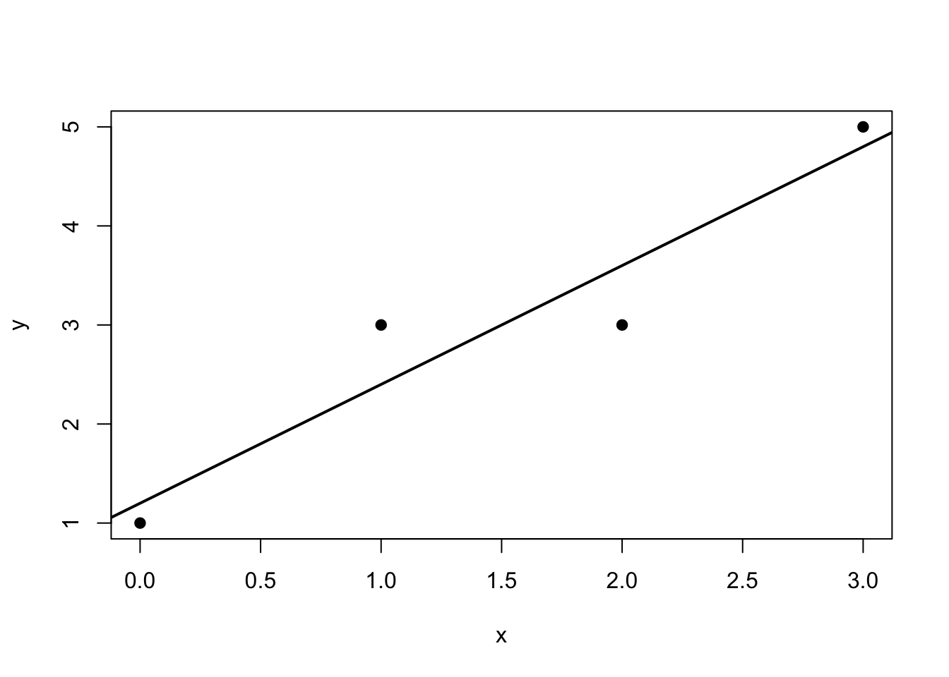
9. Worked Example by Hand
Consider the simple regression dataset
\[
\begin{array}{c|cccc}
x_i & 0 & 1 & 2 & 3 \\
\hline
y_i & 1 & 3 & 3 & 5
\end{array}
\]
Then
\[
\mathbf{Y}
=
\begin{bmatrix}
1 \\ 3 \\ 3 \\ 5
\end{bmatrix},
\qquad
\mathbf{X}
=
\begin{bmatrix}
1 & 0 \\
1 & 1 \\
1 & 2 \\
1 & 3
\end{bmatrix}.
\]
First compute
\[
\mathbf{X}^\top \mathbf{X}
=
\begin{bmatrix}
4 & 6 \\
6 & 14
\end{bmatrix},
\qquad
\mathbf{X}^\top \mathbf{Y}
=
\begin{bmatrix}
12 \\
24
\end{bmatrix}.
\]
Hence,
\[
\hat{\boldsymbol{\beta}}
=
(\mathbf{X}^\top \mathbf{X})^{-1}\mathbf{X}^\top \mathbf{Y}.
\]
Since
\[
(\mathbf{X}^\top \mathbf{X})^{-1}
=
\frac{1}{20}
\begin{bmatrix}
14 & -6 \\
-6 & 4
\end{bmatrix},
\]
we obtain
\[
\hat{\boldsymbol{\beta}}
=
\frac{1}{20}
\begin{bmatrix}
14 & -6 \\
-6 & 4
\end{bmatrix}
\begin{bmatrix}
12 \\
24
\end{bmatrix}
=
\begin{bmatrix}
1.2 \\
1.2
\end{bmatrix}.
\]
Thus, the fitted line is
\[
\hat{Y} = 1.2 + 1.2x.
\]
10. R Demonstration
10.1 Fit the model
<- c (0 , 1 , 2 , 3 )<- c (1 , 3 , 3 , 5 )<- lm (y ~ x)coef (fit)
  (Intercept) x
1           1 0
2           1 1
3           1 2
4           1 3
attr(,"assign")
[1] 0 1
<- matrix (y, ncol = 1 )<- solve (t (X) %*% X) %*% t (X) %*% Y
            [,1]
(Intercept)  1.2
x            1.2
<- X %*% beta_hat<- Y - y_hat
  [,1]
1  1.2
2  2.4
3  3.6
4  4.8
  [,1]
1 -0.2
2  0.6
3 -0.6
4  0.2
<- X %*% solve (t (X) %*% X) %*% t (X)round (H, 4 )
     1   2   3    4
1  0.7 0.4 0.1 -0.2
2  0.4 0.3 0.2  0.1
3  0.1 0.2 0.3  0.4
4 -0.2 0.1 0.4  0.7
  1 2 3 4
1 0 0 0 0
2 0 0 0 0
3 0 0 0 0
4 0 0 0 0
  1 2 3 4
1 0 0 0 0
2 0 0 0 0
3 0 0 0 0
4 0 0 0 0
plot (x, y, pch = 19 , xlab = "x" , ylab = "y" )abline (fit, lwd = 2 )
Interpretation of the Geometry
The vector \(\mathbf{Y}\) lives in \(\mathbb{R}^n\) . The model space \(\mathcal{C}(\mathbf{X})\) is a \(p\) -dimensional subspace of \(\mathbb{R}^n\) when \(\mathbf{X}\) has full rank.
Least squares finds the point in this subspace that is closest to \(\mathbf{Y}\) .
This is why • fitted values are projections, • residuals are orthogonal to the model space, • sum of squares decompositions are geometric identities.
In-Class Discussion Questions
Why does minimizing \(|\mathbf{Y} - \mathbf{X}\boldsymbol{\beta}|^2\) lead to orthogonality?
Why is the hat matrix called a projection matrix?
Why does the inclusion of an intercept imply that the residuals sum to zero?
What fails when \(\mathbf{X}\) does not have full column rank?
Practice Problems
Conceptual 1. Explain why \(\mathbf{X}^\top \mathbf{e} = \mathbf{0}\) is a geometric statement. 2. Give an interpretation of \(\mathcal{C}(\mathbf{X})\) in the context of regression. 3. Explain the difference between \(\mathbf{H}\) and \(\mathbf{M} = \mathbf{I}_n - \mathbf{H}\) .
Computational
Let
\[
\mathbf{X}
=
\begin{bmatrix}
1 & 0 \
1 & 1 \
1 & 2
\end{bmatrix},
\qquad
\mathbf{Y}
=
\begin{bmatrix}
1 \
2 \
2
\end{bmatrix}.
\]
Compute \(\mathbf{X}^\top \mathbf{X}\) .
Compute \(\mathbf{X}^\top \mathbf{Y}\) .
Find \(\hat{\boldsymbol{\beta}}\) .
Compute \(\hat{\mathbf{Y}}\) and \(\mathbf{e}\) .
Verify that \(\mathbf{X}^\top \mathbf{e} = \mathbf{0}\) .
Proof-based
Show that the hat matrix
\[
\mathbf{H} = \mathbf{X}(\mathbf{X}^\top \mathbf{X})^{-1}\mathbf{X}^\top
\]
is symmetric and idempotent.
Suggested Homework
Complete the following tasks:
derive the normal equations from the least squares criterion;
prove that \(\hat{\mathbf{Y}}\) is the projection of \(\mathbf{Y}\) onto \(\mathcal{C}(\mathbf{X})\) ;
prove that \(\mathbf{X}^\top \mathbf{e} = \mathbf{0}\) ;
verify that \(\mathbf{H}\) is symmetric and idempotent;
fit a simple regression model in R and compute: + \(\hat{\boldsymbol{\beta}}\) , + \(\hat{\mathbf{Y}}\) , + \(\mathbf{e}\) , • \(\mathbf{H}\) .
Summary
In this week, we introduced the least squares estimator and showed that it solves the normal equations
\[
\mathbf{X}^\top \mathbf{X}\hat{\boldsymbol{\beta}} = \mathbf{X}^\top \mathbf{Y}.
\]
When \(\mathbf{X}\) has full column rank,
\[
\hat{\boldsymbol{\beta}}
=
(\mathbf{X}^\top \mathbf{X})^{-1}\mathbf{X}^\top \mathbf{Y}.
\]
Geometrically, least squares is projection onto the column space of \(\mathbf{X}\) . This leads naturally to the hat matrix, residual orthogonality, and sum of squares decompositions.
Next week, we will study the distribution theory of OLS under the normal error model, including estimation of \(\sigma^2\) , standard errors, and inference.
Appendix: Matrix Calculus Facts Used This Week
For a vector \(\boldsymbol{\beta}\) and constant matrix \(\mathbf{A}\) ,
\[
\frac{\partial}{\partial \boldsymbol{\beta}}
(\mathbf{a}^\top \boldsymbol{\beta})
=
\mathbf{a},
\]
and if \(\mathbf{A}\) is symmetric,
\[
\frac{\partial}{\partial \boldsymbol{\beta}}
(\boldsymbol{\beta}^\top \mathbf{A}\boldsymbol{\beta})
=
2\mathbf{A}\boldsymbol{\beta}.
\]
These identities justify the derivative of the least squares criterion.