1  Introduction

This is an introduction to the course for linear statistical analysis. It will give you an overview of what we will be covering in the course and how to get the most out of it. We will be covering a wide range of topics in linear statistical analysis, including linear regression, generalized linear models, and mixed effects models. We will also be discussing the assumptions underlying these models and how to check them.

The course will be structured around lectures, homework assignments, and a final project. The lectures will cover the theoretical aspects of the material, while the homework assignments will give you the opportunity to apply what you have learned to real data sets. The final project will allow you to explore a topic of your choice in more depth and present your findings to the class.

To get the most out of this course, it is important to attend all lectures and complete all homework assignments. It is also important to ask questions and participate in class discussions. The more you engage with the material, the more you will learn.

I am looking forward to a great semester and I hope you are too!

To illustrate the concepts we will be covering in this course, let’s consider a simple example. Suppose we have a data set of heights and weights of individuals. We want to understand the relationship between height and weight, and we can use linear regression to model this relationship.

# Load necessary libraries
library(ggplot2)
library(dplyr)
# Create a sample data set
set.seed(123)

theme_set(theme_minimal())

n <- 100
heights <- rnorm(n, mean = 170, sd = 10)
weights <- 0.5 * heights + rnorm(n, mean = 0, sd
 = 5)
data <- data.frame(heights, weights)
# Fit a linear regression model
model <- lm(weights ~ heights, data = data)
# Summarize the model
summary(model)

Call:
lm(formula = weights ~ heights, data = data)

Residuals:
    Min      1Q  Median      3Q     Max 
-9.5367 -3.4175 -0.4375  2.9032 16.4520 

Coefficients:
            Estimate Std. Error t value Pr(>|t|)    
(Intercept)  3.94607    9.14588   0.431    0.667    
heights      0.47376    0.05344   8.865  3.5e-14 ***
---
Signif. codes:  0 '***' 0.001 '**' 0.01 '*' 0.05 '.' 0.1 ' ' 1

Residual standard error: 4.854 on 98 degrees of freedom
Multiple R-squared:  0.4451,    Adjusted R-squared:  0.4394 
F-statistic:  78.6 on 1 and 98 DF,  p-value: 3.497e-14

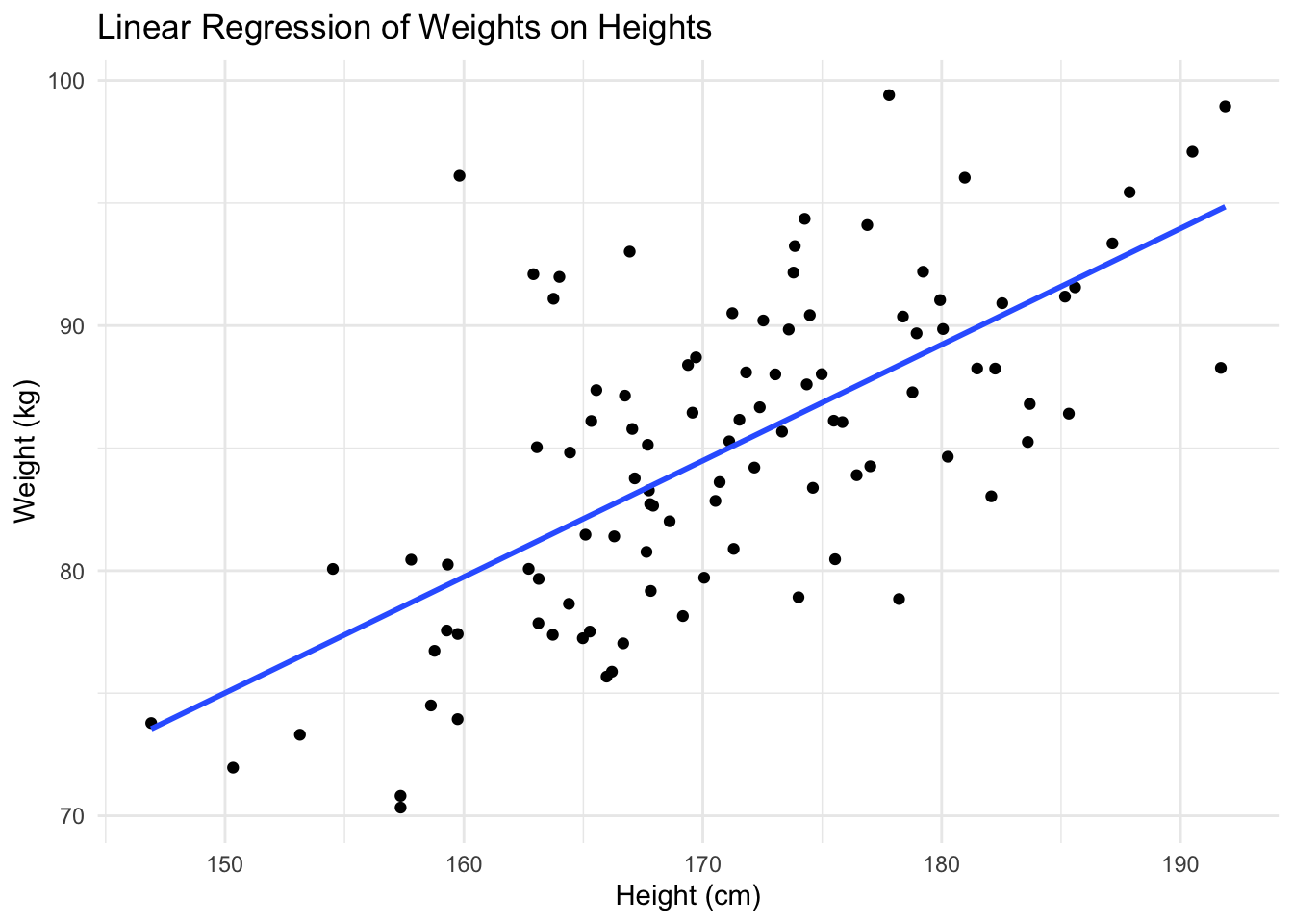
# Plot the data and the fitted line
ggplot(data, aes(x = heights, y = weights)) +
  geom_point() +
  geom_smooth(method = "lm", se = FALSE) +
  labs(title = "Linear Regression of Weights on Heights",
       x = "Height (cm)",
       y = "Weight (kg)")

`geom_smooth()` using formula = 'y ~ x'

In this example, we generated a data set of heights and weights, fitted a linear regression model to the data, and visualized the relationship between height and weight. This is just a simple example, but it illustrates the types of analyses we will be doing in this course. We will be covering much more complex models and data sets as we progress through the semester.