6  Week 5: Multiple Regression, Partial Effects, and Categorical Predictors

In this week, we move from simple regression ideas to multiple regression. We study how regression coefficients are interpreted when several predictors are included in the model, how categorical predictors enter through indicator variables, and how interactions change the meaning of coefficients. The main goal is to help students read, build, and interpret regression models in realistic settings.

6.1 Learning Objectives

By the end of this week, students should be able to:

• interpret coefficients in a multiple regression model;
• explain the meaning of a partial regression coefficient;
• distinguish between marginal association and adjusted association;
• incorporate categorical predictors using indicator variables;
• interpret regression models with interactions;
• use software output to explain fitted multiple regression models.

6.2 Reading

Recommended reading for this week:

• Seber and Lee:
  • sections on multiple linear regression
  • interpretation of regression coefficients
  • indicator variables and model formulation
• Montgomery, Peck, and Vining:
  • sections on multiple regression
  • qualitative predictors
  • interaction terms and interpretation

6.3 Review of the Regression Framework

Recall the linear model

\[ \mathbf{Y} = \mathbf{X}\boldsymbol{\beta} + \boldsymbol{\varepsilon}, \qquad \boldsymbol{\varepsilon} \sim N_n(\mathbf{0}, \sigma^2 \mathbf{I}_n). \]

When the design matrix \(\mathbf{X}\) has full column rank, the ordinary least squares estimator is

\[ \hat{\boldsymbol{\beta}} = (\mathbf{X}^\top \mathbf{X})^{-1}\mathbf{X}^\top \mathbf{Y}. \]

In earlier weeks, we focused on estimation, inference, ANOVA decomposition, and the comparison of nested models. In this week, the emphasis shifts toward interpretation and modelling structure.

6.4 From Simple Regression to Multiple Regression

In simple linear regression, we write

\[ Y_i = \beta_0 + \beta_1 x_i + \varepsilon_i. \]

Here, the slope \(\beta_1\) measures the expected change in the response associated with a one-unit increase in \(x\).

In multiple regression, the model becomes

\[ Y_i = \beta_0 + \beta_1 x_{i1} + \beta_2 x_{i2} + \cdots + \beta_p x_{ip} + \varepsilon_i. \]

Now each coefficient must be interpreted while holding the other predictors fixed.

This is the key conceptual shift.

6.5 Why Multiple Regression Matters

Multiple regression is important because real data usually involve several explanatory variables.

Reasons for including multiple predictors include:

• improving prediction;
• adjusting for confounding variables;
• estimating the effect of one variable while controlling for others;
• allowing more realistic scientific interpretation.

A coefficient in multiple regression is therefore usually an adjusted effect, not a purely marginal one.

6.6 Interpreting the Intercept

In the model

\[ Y_i = \beta_0 + \beta_1 x_{i1} + \beta_2 x_{i2} + \cdots + \beta_p x_{ip} + \varepsilon_i, \]

the intercept \(\beta_0\) is the expected value of the response when all predictors equal zero:

\[ \mathbb{E}[Y_i \mid x_{i1}, \dots, x_{ip}] = \beta_0 \quad \text{when } x_{i1} = \cdots = x_{ip} = 0. \]

This interpretation may or may not be scientifically meaningful.

Sometimes zero is a natural baseline. Sometimes it is outside the observed range, in which case the intercept is mainly a mathematical anchor for the model.

6.7 Interpreting Partial Regression Coefficients

Consider the model

\[ Y_i = \beta_0 + \beta_1 x_{i1} + \beta_2 x_{i2} + \varepsilon_i. \]

Then:

• \(\beta_1\) is the expected change in \(Y\) associated with a one-unit increase in \(x_1\), holding \(x_2\) fixed;
• \(\beta_2\) is the expected change in \(Y\) associated with a one-unit increase in \(x_2\), holding \(x_1\) fixed.

This is called a partial effect or adjusted effect.

The phrase “holding other variables fixed” is essential and should always be stated clearly.

6.8 Marginal Association Versus Adjusted Association

Suppose \(x_1\) and \(x_2\) are correlated.

Then the relationship between \(Y\) and \(x_1\) in a simple regression of \(Y\) on \(x_1\) alone may differ from the coefficient of \(x_1\) in a multiple regression including both \(x_1\) and \(x_2\).

This happens because:

• the simple regression coefficient describes a marginal association;
• the multiple regression coefficient describes an adjusted association.

These can differ substantially when predictors are related to each other.

6.9 Example of Adjusted Interpretation

Suppose we fit

\[ \widehat{Y} = 12.5 + 0.8\,x_1 - 1.2\,x_2. \]

Then:

• for each one-unit increase in \(x_1\), the fitted mean response increases by 0.8 units, holding \(x_2\) fixed;
• for each one-unit increase in \(x_2\), the fitted mean response decreases by 1.2 units, holding \(x_1\) fixed.

This interpretation is valid only within the modelling assumptions and over the range of data where the model is reasonable.

6.10 Matrix View of Multiple Regression

In multiple regression, the design matrix has the form

\[ \mathbf{X} = \begin{bmatrix} 1 & x_{11} & x_{12} & \cdots & x_{1p} \\ 1 & x_{21} & x_{22} & \cdots & x_{2p} \\ \vdots & \vdots & \vdots & \ddots & \vdots \\ 1 & x_{n1} & x_{n2} & \cdots & x_{np} \end{bmatrix}. \]

Each column corresponds to a predictor or model term.

This allows the same least squares and inference framework to handle:

• continuous predictors;
• categorical predictors represented by indicator variables;
• interactions;
• polynomial terms.

So the general linear model framework is highly flexible.

6.11 Categorical Predictors and Indicator Variables

Many real predictors are categorical rather than numeric.

Examples include:

• treatment group;
• sex;
• school type;
• region;
• machine type.

These enter a regression model through indicator variables, also called dummy variables.

6.12 Binary Predictor

Suppose \(z_i\) is a binary variable:

\[ z_i = \begin{cases} 1, & \text{if observation } i \text{ is in group A}, \\ 0, & \text{if observation } i \text{ is in group B}. \end{cases} \]

Then the model

\[ Y_i = \beta_0 + \beta_1 z_i + \varepsilon_i \]

has the following interpretation:

• when \(z_i = 0\), the expected response is \(\beta_0\);
• when \(z_i = 1\), the expected response is \(\beta_0 + \beta_1\).

Thus, \(\beta_1\) measures the difference in group means.

6.13 More Than Two Categories

Suppose a categorical predictor has three levels:

• A,
• B,

We usually represent it with two indicator variables, for example:

\[ z_{1i} = \begin{cases} 1, & \text{if level B},\\ 0, & \text{otherwise}, \end{cases} \qquad z_{2i} = \begin{cases} 1, & \text{if level C},\\ 0, & \text{otherwise}. \end{cases} \]

Then level A is the reference group, and the model is

\[ Y_i = \beta_0 + \beta_1 z_{1i} + \beta_2 z_{2i} + \varepsilon_i. \]

Interpretation:

• level A mean: \(\beta_0\);
• level B mean: \(\beta_0 + \beta_1\);
• level C mean: \(\beta_0 + \beta_2\).

So coefficients are interpreted relative to the reference category.

6.14 Why We Do Not Include All Indicators with an Intercept

If a categorical variable has \(k\) levels, then with an intercept we include only \(k-1\) indicator variables.

If we include all \(k\) indicators and also include an intercept, then the columns of the design matrix become linearly dependent. This causes rank deficiency.

This is sometimes called the dummy variable trap.

6.15 Continuous and Categorical Predictors Together

Regression models often mix continuous and categorical predictors.

For example,

\[ Y_i = \beta_0 + \beta_1 x_i + \beta_2 z_i + \varepsilon_i \]

may contain:

• a continuous predictor \(x_i\);
• a binary indicator \(z_i\).

Interpretation:

• \(\beta_1\) is the slope in \(x\) holding group fixed;
• \(\beta_2\) is the group difference holding \(x\) fixed.

This is one of the simplest forms of ANCOVA-style modelling.

6.16 Interaction Between Continuous Predictors

An interaction allows the effect of one predictor to depend on the value of another predictor.

For two continuous predictors, we may write

\[ Y_i = \beta_0 + \beta_1 x_{i1} + \beta_2 x_{i2} + \beta_3 x_{i1}x_{i2} + \varepsilon_i. \]

Now the effect of \(x_1\) is no longer constant. Instead,

\[ \frac{\partial \mathbb{E}[Y_i \mid x_{i1},x_{i2}]}{\partial x_{i1}} = \beta_1 + \beta_3 x_{i2}. \]

So the slope for \(x_1\) depends on the value of \(x_2\).

Likewise, the slope for \(x_2\) depends on \(x_1\).

6.17 Interaction Between a Continuous and a Binary Predictor

Suppose we fit

\[ Y_i = \beta_0 + \beta_1 x_i + \beta_2 z_i + \beta_3 x_i z_i + \varepsilon_i, \]

where \(z_i \in \{0,1\}\).

Then:

• when \(z_i = 0\), \[ \mathbb{E}[Y_i \mid x_i, z_i=0] = \beta_0 + \beta_1 x_i; \]

• when \(z_i = 1\), \[ \mathbb{E}[Y_i \mid x_i, z_i=1] = (\beta_0+\beta_2) + (\beta_1+\beta_3)x_i. \]

So:

• \(\beta_2\) changes the intercept;
• \(\beta_3\) changes the slope.

This allows the two groups to have different regression lines.

6.18 Main Effects in the Presence of Interaction

When an interaction is present, the meaning of the main effects changes.

For example, in

\[ Y_i = \beta_0 + \beta_1 x_i + \beta_2 z_i + \beta_3 x_i z_i + \varepsilon_i, \]

the coefficient \(\beta_1\) is the slope for \(x\) only when \(z=0\), the reference group.

Similarly, \(\beta_2\) is the group difference only when \(x=0\).

So students should be careful not to interpret main effects in isolation when interactions are included.

6.19 Centering Predictors for Interpretation

Sometimes the value zero is not meaningful for a continuous predictor.

In that case, it can be helpful to centre the predictor:

\[ x_i^* = x_i - \bar{x}. \]

Then the intercept becomes the expected response at the average value of \(x\), which may be much easier to interpret.

Centering can also improve interpretability in models with interactions.

6.20 Comparing Models With and Without Interaction

To assess whether an interaction is needed, we can compare nested models.

For example:

• reduced model: \[ Y_i = \beta_0 + \beta_1 x_i + \beta_2 z_i + \varepsilon_i; \]

• full model: \[ Y_i = \beta_0 + \beta_1 x_i + \beta_2 z_i + \beta_3 x_i z_i + \varepsilon_i. \]

The reduced model is nested within the full model by setting

\[ \beta_3 = 0. \]

So the interaction can be tested by a standard extra sum of squares \(F\) test.

6.21 Collinearity and Interpretation

In multiple regression, predictors may be strongly related to each other.

When this happens:

• coefficient estimates can become unstable;
• standard errors can become large;
• interpretation becomes more delicate.

Even when the overall model seems useful, individual coefficients may be hard to estimate precisely.

This issue is called multicollinearity.

We will study diagnostics for it more formally later, but students should already know that “holding other variables fixed” may become practically difficult if predictors tend to move together.

6.22 Multiple Regression as Conditional Mean Modelling

A good way to summarize multiple regression is:

\[ \mathbb{E}[Y \mid X_1,\dots,X_p] \]

is being modelled as a linear function of predictors and model terms.

This viewpoint helps unify:

• continuous predictors;
• factors;
• interactions;
• transformed predictors.

It also helps students distinguish between the response itself and its conditional mean.

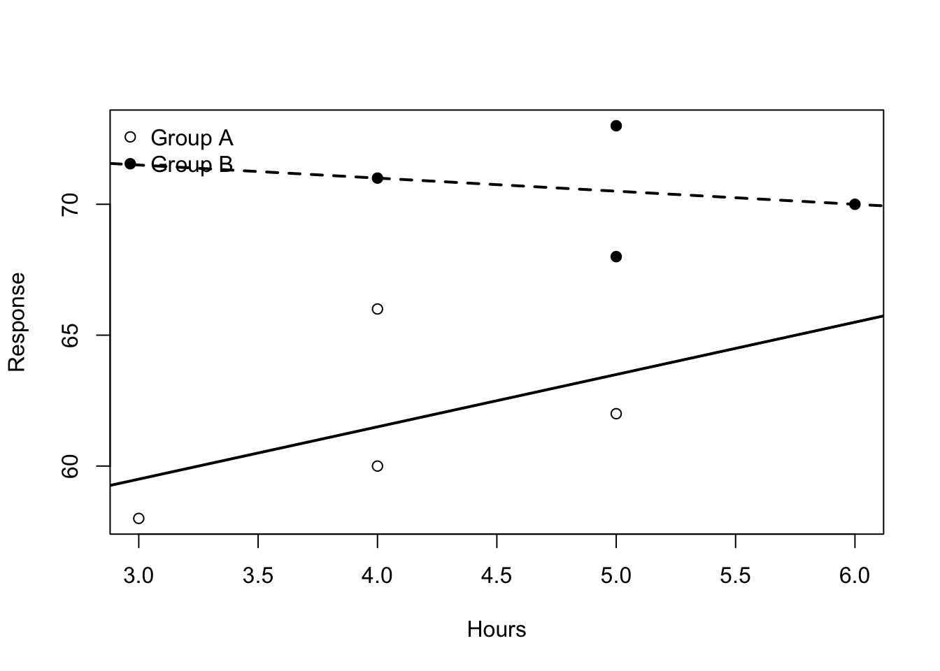
6.23 Worked Example With a Continuous and a Binary Predictor

Suppose we observe a response \(Y\), a study-hours variable \(x\), and a tutoring indicator \(z\), where

• \(z=0\) means no tutoring;
• \(z=1\) means tutoring.

Consider the model

\[ Y_i = \beta_0 + \beta_1 x_i + \beta_2 z_i + \varepsilon_i. \]

Suppose the fitted equation is

\[ \hat{Y} = 50 + 3x + 8z. \]

Then:

• among students with the same tutoring status, one extra hour of study is associated with an increase of 3 points in the fitted mean score;
• among students with the same number of study hours, the tutoring group has a fitted mean score 8 points higher than the non-tutoring group.

If we add an interaction and obtain

\[ \hat{Y} = 48 + 4x + 10z - 1.5xz, \]

then:

• for students without tutoring, the slope in study hours is 4;
• for students with tutoring, the slope in study hours is \(4 - 1.5 = 2.5\).

Thus, the effect of study time depends on tutoring status.

6.24 R Demonstration With Multiple Regression

6.25 Fit a model with two continuous predictors

dat1 <- data.frame(
  y = c(12, 15, 14, 18, 20, 19, 23, 25),
  x1 = c(1, 2, 2, 3, 4, 4, 5, 6),
  x2 = c(5, 4, 6, 4, 3, 5, 2, 1)
)

fit1 <- lm(y ~ x1 + x2, data = dat1)
summary(fit1)

Call:
lm(formula = y ~ x1 + x2, data = dat1)

Residuals:
         1          2          3          4          5          6          7 
-3.158e-01 -2.632e-02 -1.316e-01  7.105e-01  4.842e-16 -1.053e-01  2.895e-01 
         8 
-4.211e-01 

Coefficients:
            Estimate Std. Error t value Pr(>|t|)    
(Intercept)  12.2895     1.1598  10.596 0.000129 ***
x1            2.2632     0.1681  13.464 4.05e-05 ***
x2           -0.4474     0.1697  -2.636 0.046186 *  
---
Signif. codes:  0 '***' 0.001 '**' 0.01 '*' 0.05 '.' 0.1 ' ' 1

Residual standard error: 0.423 on 5 degrees of freedom
Multiple R-squared:  0.9936,    Adjusted R-squared:  0.991 
F-statistic: 387.3 on 2 and 5 DF,  p-value: 3.295e-06

6.26 Compare with a simple regression

fit1_simple <- lm(y ~ x1, data = dat1)
summary(fit1_simple)

Call:
lm(formula = y ~ x1, data = dat1)

Residuals:
     Min       1Q   Median       3Q      Max 
-0.89308 -0.27201  0.05031  0.39308  0.73585 

Coefficients:
            Estimate Std. Error t value Pr(>|t|)    
(Intercept)   9.3774     0.4988   18.80 1.46e-06 ***
x1            2.6289     0.1339   19.63 1.13e-06 ***
---
Signif. codes:  0 '***' 0.001 '**' 0.01 '*' 0.05 '.' 0.1 ' ' 1

Residual standard error: 0.597 on 6 degrees of freedom
Multiple R-squared:  0.9847,    Adjusted R-squared:  0.9821 
F-statistic: 385.4 on 1 and 6 DF,  p-value: 1.132e-06

summary(fit1)

Call:
lm(formula = y ~ x1 + x2, data = dat1)

Residuals:
         1          2          3          4          5          6          7 
-3.158e-01 -2.632e-02 -1.316e-01  7.105e-01  4.842e-16 -1.053e-01  2.895e-01 
         8 
-4.211e-01 

Coefficients:
            Estimate Std. Error t value Pr(>|t|)    
(Intercept)  12.2895     1.1598  10.596 0.000129 ***
x1            2.2632     0.1681  13.464 4.05e-05 ***
x2           -0.4474     0.1697  -2.636 0.046186 *  
---
Signif. codes:  0 '***' 0.001 '**' 0.01 '*' 0.05 '.' 0.1 ' ' 1

Residual standard error: 0.423 on 5 degrees of freedom
Multiple R-squared:  0.9936,    Adjusted R-squared:  0.991 
F-statistic: 387.3 on 2 and 5 DF,  p-value: 3.295e-06

6.27 Fit a model with a categorical predictor

dat2 <- data.frame(
  y = c(60, 62, 58, 71, 73, 70, 66, 68),
  hours = c(4, 5, 3, 4, 5, 6, 4, 5),
  group = factor(c("A", "A", "A", "B", "B", "B", "A", "B"))
)

fit2 <- lm(y ~ hours + group, data = dat2)
summary(fit2)

Call:
lm(formula = y ~ hours + group, data = dat2)

Residuals:
    1     2     3     4     5     6     7     8 
-1.50 -0.25 -2.75  1.25  2.50 -1.25  4.50 -2.50 

Coefficients:
            Estimate Std. Error t value Pr(>|t|)    
(Intercept)   58.500      6.236   9.381 0.000232 ***
hours          0.750      1.512   0.496 0.641001    
groupB         8.250      2.620   3.149 0.025399 *  
---
Signif. codes:  0 '***' 0.001 '**' 0.01 '*' 0.05 '.' 0.1 ' ' 1

Residual standard error: 3.025 on 5 degrees of freedom
Multiple R-squared:  0.7821,    Adjusted R-squared:  0.695 
F-statistic: 8.975 on 2 and 5 DF,  p-value: 0.02215

model.matrix(fit2)

  (Intercept) hours groupB
1           1     4      0
2           1     5      0
3           1     3      0
4           1     4      1
5           1     5      1
6           1     6      1
7           1     4      0
8           1     5      1
attr(,"assign")
[1] 0 1 2
attr(,"contrasts")
attr(,"contrasts")$group
[1] "contr.treatment"

6.28 Fit a model with interaction

fit3 <- lm(y ~ hours * group, data = dat2)
summary(fit3)

Call:
lm(formula = y ~ hours * group, data = dat2)

Residuals:
         1          2          3          4          5          6          7 
-1.500e+00 -1.500e+00 -1.500e+00 -2.216e-15  2.500e+00 -7.730e-16  4.500e+00 
         8 
-2.500e+00 

Coefficients:
             Estimate Std. Error t value Pr(>|t|)   
(Intercept)    53.500      9.026   5.927  0.00406 **
hours           2.000      2.222   0.900  0.41897   
groupB         19.500     14.401   1.354  0.24715   
hours:groupB   -2.500      3.142  -0.796  0.47083   
---
Signif. codes:  0 '***' 0.001 '**' 0.01 '*' 0.05 '.' 0.1 ' ' 1

Residual standard error: 3.142 on 4 degrees of freedom
Multiple R-squared:  0.8119,    Adjusted R-squared:  0.6708 
F-statistic: 5.755 on 3 and 4 DF,  p-value: 0.06202

anova(fit2, fit3)

Analysis of Variance Table

Model 1: y ~ hours + group
Model 2: y ~ hours * group
  Res.Df   RSS Df Sum of Sq      F Pr(>F)
1      5 45.75                           
2      4 39.50  1      6.25 0.6329 0.4708

6.29 Plot group-specific regression lines

plot(dat2$hours, dat2$y,
     pch = ifelse(dat2$group == "A", 1, 19),
     xlab = "Hours",
     ylab = "Response")
abline(a = coef(fit3)[1], b = coef(fit3)[2], lwd = 2)
abline(a = coef(fit3)[1] + coef(fit3)[3],
       b = coef(fit3)[2] + coef(fit3)[4],
       lwd = 2, lty = 2)
legend("topleft", legend = c("Group A", "Group B"),
       pch = c(1, 19), bty = "n")

6.30 Interpreting Software Output

In summary(lm(...)), each coefficient estimate answers a question about the conditional mean given the model terms included.

Students should always ask:

• what variables are being held fixed;
• what is the reference category;
• whether an interaction changes the meaning of the main effects;
• whether zero is a meaningful baseline for interpretation.

These questions matter more than memorizing formulas.

6.31 In-Class Discussion Questions

1. Why can the coefficient of a predictor change when a second predictor is added to the model?
2. Why do we need a reference category for categorical predictors?
3. How does an interaction change the interpretation of a main effect?
4. When might centring a predictor improve interpretation?

6.32 Practice Problems

6.33 Conceptual

1. Explain the meaning of a partial regression coefficient in your own words.
2. Explain the difference between a marginal association and an adjusted association.
3. Explain why a model with an interaction requires more careful interpretation than an additive model.

6.34 Computational

Suppose the fitted model is

\[ \hat{Y} = 10 + 2x_1 - 3x_2. \]

1. Interpret the coefficient of \(x_1\).
2. Interpret the coefficient of \(x_2\).
3. Compute the fitted mean response when \(x_1 = 4\) and \(x_2 = 1\).

Now suppose the fitted model is

\[ \hat{Y} = 20 + 5x + 7z - 2xz, \]

where \(z\) is binary.

1. Write the fitted mean function when \(z=0\).
2. Write the fitted mean function when \(z=1\).
3. Interpret the interaction coefficient.

6.35 Indicator Variable Problem

A factor has four levels: A, B, C, and D.

1. How many indicator variables are needed if the model includes an intercept?
2. If A is the reference group, write a regression model using indicators for B, C, and D.
3. State the expected response for each group.

6.36 Suggested Homework

Complete the following tasks:

• fit a multiple regression model with at least two continuous predictors and interpret all coefficients;
• fit a model with one continuous predictor and one categorical predictor, then identify the reference category and explain all coefficients;
• add an interaction term and compare the additive and interaction models;
• use model.matrix() in R to inspect the design matrix for a model with factors;
• write a short explanation of why coefficient interpretation changes when additional predictors are added.

6.37 Summary

In this week, we developed the interpretation of multiple regression models.

We emphasized that:

• regression coefficients in multiple regression are partial effects;
• categorical predictors are incorporated through indicator variables;
• interactions allow the effect of one predictor to depend on another;
• the meaning of a coefficient depends on the full model specification.

These ideas are essential for moving from formal least squares theory to practical statistical modelling.

Next week, a natural continuation is to study multicollinearity, variable selection, and model building, or to move into diagnostics and residual analysis, depending on the course emphasis.

6.38 Appendix: Compact Interpretation Guide

For the additive model

\[ Y = \beta_0 + \beta_1 x_1 + \beta_2 x_2 + \varepsilon, \]

• \(\beta_0\): expected response when \(x_1=x_2=0\);
• \(\beta_1\): expected change in response for a one-unit increase in \(x_1\), holding \(x_2\) fixed;
• \(\beta_2\): expected change in response for a one-unit increase in \(x_2\), holding \(x_1\) fixed.

For the model with a binary predictor

\[ Y = \beta_0 + \beta_1 x + \beta_2 z + \varepsilon, \]

• \(\beta_0\): mean for the reference group when \(x=0\);
• \(\beta_1\): slope in \(x\) for fixed group;
• \(\beta_2\): group difference for fixed \(x\).

For the interaction model

\[ Y = \beta_0 + \beta_1 x + \beta_2 z + \beta_3 xz + \varepsilon, \]

• slope in \(x\) when \(z=0\): \(\beta_1\);
• slope in \(x\) when \(z=1\): \(\beta_1+\beta_3\);
• group difference when \(x=0\): \(\beta_2\).