6 Contrasts and Estimable Comparisons

A scientific question often concerns a difference between means rather than one coefficient printed by software. This chapter uses the linear-combination inference from Chapter 3 — Distribution Theory of OLS and Inference to express those questions. Chapter 7 — Experimental Design Models: ANOVA and ANCOVA connects these comparisons to experimental designs.

Learning objectives. Express a comparison of group means as a linear function of regression coefficients, obtain its estimate and interval, and distinguish a meaningful comparison from a coding-dependent coefficient.

6.1 Comparisons of group means

Suppose the conditional means of three groups are \(\mu_A\), \(\mu_B\), and \(\mu_C\). A question such as “Does A differ from the average of B and C?” concerns \(\theta=\mu_A-(\mu_B+\mu_C)/2\).

Definition 6.1 (Contrast of Group Means) A contrast is a linear combination \(\theta=\sum_{j=1}^g c_j\mu_j\) whose weights satisfy \(\sum_{j=1}^g c_j=0\). The zero-sum condition makes the comparison unchanged when the same constant is added to every group mean.

From means to coefficients. With A as the reference group, write \(\boldsymbol{\beta}=(\beta_0,\beta_B,\beta_C)^\top\). Then \(\mu_A=\beta_0\), \(\mu_B=\beta_0+\beta_B\), and \(\mu_C=\beta_0+\beta_C\), so

\[ \theta=-\tfrac12\beta_B-\tfrac12\beta_C =\mathbf{a}^\top\boldsymbol{\beta},\qquad \mathbf{a}=(0,-\tfrac12,-\tfrac12)^\top. \]

The zero-sum condition applies to mean weights

The weights on \((\mu_A,\mu_B,\mu_C)\) sum to zero. The equivalent weights on treatment-coded regression coefficients need not sum to zero. Always translate the scientific comparison through the chosen parameterization.

Under the full-rank normal linear model, use

\[ \hat\theta=\mathbf{a}^\top\hat{\boldsymbol{\beta}},\qquad \operatorname{SE}(\hat\theta)=\hat\sigma \sqrt{\mathbf{a}^\top(\mathbf{X}^\top\mathbf{X})^{-1}\mathbf{a}}. \]

A confidence interval is \(\hat\theta\pm t_{1-\alpha/2,n-p}\operatorname{SE}(\hat\theta)\). This is the same procedure as in Chapter 3 — Distribution Theory of OLS and Inference, applied to a different target. Several independent restrictions can be collected into \(C\beta=d\), with \(\operatorname{rank}(C)=r\), and tested jointly using the general F test.

Interpretation. Report the contrast estimate in the units of the response, its interval, and which population means it compares. Equality of two slopes is only a meaningful scientific question when their units and scales make that comparison defensible.

6.2 Coding and estimability

Changing the reference group changes the coefficient labels and values, but not the fitted group means or a fixed comparison of those means. The vector \(\mathbf{a}\) must change with the coding so that it represents the same target.

Example 6.1 (An Intercept and All Group Indicators) In \(Y_{ij}=\mu+\tau_i+\varepsilon_{ij}\), adding a constant to every \(\tau_i\) and subtracting it from \(\mu\) leaves every group mean unchanged. The separate parameters are not identified without a constraint, but \(\tau_A-\tau_B\) is unchanged and is estimable.

The practical lesson is to state the target in terms of observable mean responses before reading coefficients. For the row-space criterion and generalized-inverse formulation, see Linear-Model Extensions (Optional).

One comparison versus a family of comparisons

A single prespecified contrast and a search through many contrasts are different inferential procedures. Define the family being reported. For all pairwise group comparisons, Tukey intervals are useful; for a specified family of tests, Holm adjustment is another option. An omnibus F test does not automatically justify every unadjusted pairwise test.

6.3 A complete contrast analysis in R

This simulated example separates the known data-generating means from their noisy estimates. Changing the seed changes the sample, not the target comparison.

Show R code

library(ggplot2)
theme_set(theme_minimal(base_size = 11) +
            theme(legend.position = "bottom",
              panel.grid.minor = element_blank()))

set.seed(8561)
group <- factor(rep(c("A", "B", "C"), each = 12))
mu <- c(A = 10, B = 13, C = 15)
dat <- data.frame(group,
                  y = unname(mu[group]) + rnorm(length(group), sd = 2))
fit <- lm(y ~ group, data = dat)

# A minus the average of B and C, under treatment coding.
a <- c(0, -1/2, -1/2)
estimate <- sum(a * coef(fit))
se <- sqrt(drop(t(a) %*% vcov(fit) %*% a))
df <- df.residual(fit)
ci <- estimate + c(-1, 1) * qt(0.975, df) * se
c(estimate = estimate, SE = se, lower = ci[1], upper = ci[2],
  p_value = 2 * pt(-abs(estimate / se), df))

     estimate            SE         lower         upper       p_value
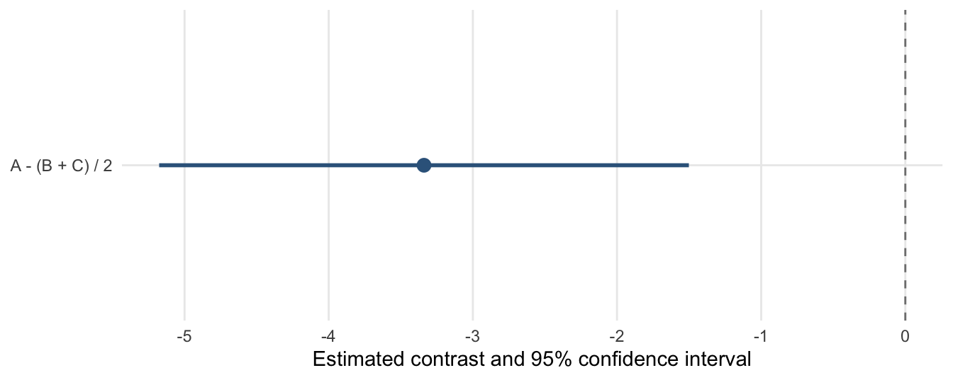
-3.3388312952  0.9030487544 -5.1760978004 -1.5015647901  0.0007874472

Verify the same question under another coding. A cell-means model directly estimates \((\mu_A,\mu_B,\mu_C)\), so its contrast weights are \((1,-1/2,-1/2)\).

Show R code

fit_means <- lm(y ~ 0 + group, data = dat)
c_mean <- c(1, -1/2, -1/2)
estimate_means <- sum(c_mean * coef(fit_means))
se_means <- sqrt(drop(t(c_mean) %*% vcov(fit_means) %*% c_mean))
rbind(treatment_coding = c(estimate, se),
      cell_means_coding = c(estimate_means, se_means))

                       [,1]      [,2]
treatment_coding  -3.338831 0.9030488
cell_means_coding -3.338831 0.9030488

Show R code

contrast_result <- data.frame(estimate, lower = ci[1], upper = ci[2],
                               comparison = "A - (B + C) / 2")
ggplot(contrast_result, aes(estimate, comparison)) +
  geom_vline(xintercept = 0, linetype = "dashed", colour = "grey50") +
  geom_segment(aes(x = lower, xend = upper, yend = comparison),
               linewidth = 1, colour = "steelblue4") +
  geom_point(size = 3, colour = "steelblue4") +
  expand_limits(x = 0) +
  labs(x = "Estimated contrast and 95% confidence interval", y = NULL)

Figure 6.1: The estimated A-minus-average-of-B-and-C contrast and its 95% confidence interval. Zero represents no difference for this particular comparison.

A family of comparisons. For all three pairwise group differences, fit the one-way ANOVA and request simultaneous Tukey intervals:

Show R code

TukeyHSD(aov(y ~ group, data = dat))

  Tukey multiple comparisons of means
    95% family-wise confidence level

Fit: aov(formula = y ~ group, data = dat)

$group
         diff        lwr      upr     p adj
B-A 2.8862540  0.3275576 5.444950 0.0242654
C-A 3.7914086  1.2327122 6.350105 0.0026175
C-B 0.9051546 -1.6535418 3.463851 0.6639004

These intervals answer a different collection of questions from the single contrast above. Do not infer a difference between group means by inspecting whether two separate mean-response intervals overlap.

6.4 Practice

Express \(\mu_B-\mu_C\) under treatment coding with A as reference, then under cell-means coding.
Verify that the estimate and standard error agree under the two codings.
Explain why the coefficients can change after changing the reference group while the scientific comparison remains unchanged.
Specify the comparison family before reporting all pairwise differences, and explain the role of multiplicity adjustment.