5 Monte Carlo Simulation and Variance Reduction

In Chapter 4, we learned to generate random values. Here we use them to answer a question about a probability model.

The key questions are conceptual:

Why simulate? The answer may be hard to calculate directly.
What do we do? Generate possible inputs, calculate their outputs, and summarize.
Where does variation come from? Fresh random inputs give a different set of outputs and a different estimate.
What does variance reduction change? It makes the estimate more stable while keeping the same target.

We begin with a shop deciding how many muffins to prepare, then use \(\mathbb{E}[e^U]\) with \(U\sim\operatorname{Uniform}(0,1)\) to compare variance-reduction methods. Detailed formulas, proofs, and extra examples are in Supplementary.

5.1 The Main Idea: Simulate, Calculate, Average

5.1.1 Why use simulation?

Suppose a model describes uncertain inputs, and we want its average output or the probability of an event. An exact calculation may involve a difficult integral or many inputs. If we can generate inputs from the model and calculate the corresponding outputs, simulation gives us a practical numerical estimate.

Simulation uses computer-generated outcomes to explore a specified model. More simulated outcomes improve numerical precision; they do not supply new real observations or make the model more realistic.

5.1.2 What happens in one run?

One draw produces one input and its output. One run repeats this process \(N\) times and reports one estimate:

Simulate: draw an input \(X_i\) from the specified probability model.
Calculate: use the model to obtain \(Y_i=g(X_i)\).
Average: repeat independently and average the \(N\) outputs.

\[ \theta=\mathbb{E}[g(X)], \qquad \widehat\theta=\frac{1}{N}\sum_{i=1}^N Y_i. \]

Here \(\theta\) is the fixed answer we want and \(\widehat\theta\) is the answer from this run. A contribution simply means one value \(Y_i\) going into the average.

5.1.3 A Practical Example: Are 12 Muffins Enough?

The question. A shop prepares 12 muffins each morning. What is the probability that demand exceeds the stock, so at least one customer cannot buy a muffin?

For this teaching example, assume 20 potential customers per day. Each independently wants one muffin with probability 0.6, whether or not stock is available. Days are independent, and these assumptions stay the same across runs. These numbers are illustrative, not estimates from shop data.

The average demand is \(20\times0.6=12\), but an average of 12 does not mean demand is always 12. Simulation lets us try many artificial days and count how often the stock is insufficient.

Step 1: Simulate one day. For each of the 20 customers, generate a uniform number between 0 and 1. A number below 0.6 means the customer wants to buy. Count the buyers. Set the seed once here; the later steps continue the same random-number stream.

set.seed(8670)
wants_one <- runif(20) < 0.6
demand_today <- sum(wants_one)
c(demand = demand_today, insufficient = demand_today > 12)
#>       demand insufficient 
#>           10            0

This artificial day has demand 10, so the stock is sufficient. A day with demand 15 would leave 3 customers unserved. Demand 12 is still fully served: our event is demand > 12, not demand >= 12.

Step 2: Repeat for many days and record 0 or 1. Use 1 when stock is insufficient and 0 otherwise. In R, rbinom(N, size = 20, prob = 0.6) is a shortcut that generates the number of buyers for each of \(N\) independent days using exactly the same model.

N <- 1000
demand <- rbinom(N, size = 20, prob = 0.6)
insufficient <- as.integer(demand > 12)
c(days_short = sum(insufficient),
  estimated_probability = mean(insufficient))
#>            days_short estimated_probability 
#>               423.000                 0.423

Step 3: Interpret the average. Stock was insufficient on 423 of the 1,000 simulated days, giving 42.3%. That is roughly 4 days out of 10 under this model. It is an estimate of the chance for a day, not a prediction of exactly which future days will have a shortage.

Step 4: Rerun the whole experiment. Each run below simulates another 1,000 days and produces one estimated probability. Continue the random-number stream from Step 1; do not reset the seed between runs.

Repeat the 1,000-day experiment with fresh random draws

shop_large_runs <- replicate(30, {
  new_demand <- rbinom(1000, size = 20, prob = 0.6)
  mean(new_demand > 12)
})
knitr::kable(data.frame(
  Run = 1:3,
  `Simulated days` = rep(1000, 3),
  `Days with insufficient stock` = round(1000 * shop_large_runs[1:3]),
  `Estimated chance` = sprintf("%.1f%%", 100 * shop_large_runs[1:3]),
  check.names = FALSE
), booktabs = TRUE)

Run	Simulated days	Days with insufficient stock	Estimated chance
1	1000	408	40.8%
2	1000	410	41.0%
3	1000	399	39.9%

Why do the answers differ? The random buying decisions differ, so each run contains a different number of shortage days. The stock, purchase probability, and true shortage probability have not changed.

Code

shop_small_runs <- replicate(30, mean(rbinom(50, 20, 0.6) > 12))
shop_true_probability <- pbinom(12, 20, 0.6, lower.tail = FALSE)
shop_plot <- data.frame(
  Run = rep(1:30, 2),
  Estimate = c(shop_small_runs, shop_large_runs),
  Budget = factor(rep(c("50 days per run", "1,000 days per run"), each = 30),
                  levels = c("50 days per run", "1,000 days per run"))
)
ggplot(shop_plot, aes(Run, Estimate, color = Budget)) +
  geom_hline(yintercept = shop_true_probability, linetype = "dashed",
             color = "grey35") +
  geom_line(linewidth = .5, alpha = .7) +
  geom_point(size = 1.8) +
  facet_wrap(~Budget) +
  scale_color_manual(values = c("#0072B2", "#D55E00")) +
  scale_x_continuous(breaks = c(1, 10, 20, 30)) +
  scale_y_continuous(limits = c(0, 1), breaks = seq(0, 1, .25),
                    labels = function(x) paste0(100 * x, "%")) +
  labs(x = "Run number (fresh days in every run)",
       y = "Estimated chance of insufficient stock") +
  theme(legend.position = "none", strip.text = element_text(size = 12))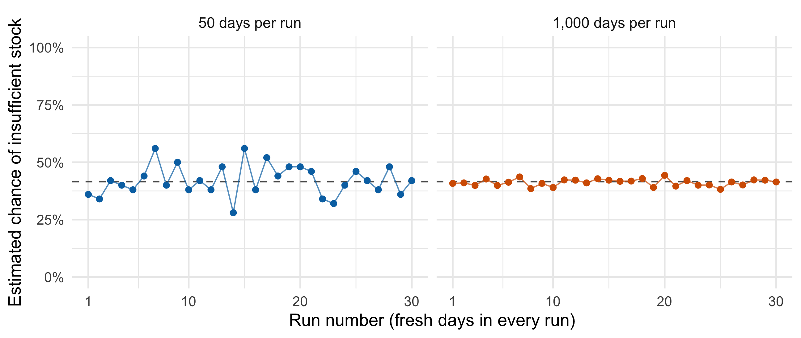

Two panels show estimated shortage probabilities across 30 runs. Estimates based on 50 days fluctuate more than estimates based on 1,000 days. Both are near the same dashed target line at 41.6 percent. — Figure 5.1: Each point is one complete simulation run, not one day. Both panels show 30 independent runs of the same shop model on the same vertical scale. Averaging 1,000 days gives a more stable estimate than averaging 50 days. The dashed line is the exact model probability, about 41.6%.

This simple model also has an exact binomial answer, about 41.6%, which checks our simulation. We practice the recipe here because it also works when the shop model becomes harder to calculate directly, such as when customers buy several items or demand changes during the day.

Two different kinds of variation

Day to day: customer demand varies. Even knowing the exact shortage probability would not tell us tomorrow’s demand.
Run to run: our estimated probability varies because each run uses only a finite number of simulated days. More simulated days reduce this numerical uncertainty; they do not make real customer demand less variable.

The practical answer is therefore: 12 muffins covers the average demand, but leaves about a 42% chance of insufficient stock under these assumptions. Choosing a stock level also requires considering shortage and leftover costs.

5.1.4 A Small Mathematical Example

Let \(U\sim\operatorname{Uniform}(0,1)\). Estimate

\[ \theta=\mathbb{E}[e^U]=\int_0^1 e^u\,du=e-1\approx1.7183. \]

The exact answer lets us check our code. In harder problems, this answer may be unavailable.

For one draw, if \(U=0.2\), the output is \(e^{0.2}\approx1.221\). This single output does not answer the average-output question; we need many draws.

set.seed(8670)
N <- 10000
u <- runif(N)              # simulate
plain_y <- exp(u)          # calculate one value per draw
c(estimate = mean(plain_y), exact = exp(1) - 1)  # average
#> estimate    exact 
#> 1.726714 1.718282

Why does averaging help? Any one draw can be unusually high or low. In a large collection, those fluctuations tend to balance, and each individual draw has less influence on the final answer.

Four boxes: choose the target, draw inputs, calculate values, and average with MCSE. — Figure 5.2: Choose the answer you want, simulate inputs, calculate one value per input, and take the average.

What to expect when you rerun the code

Fresh random draws usually give a different estimate. The model, function, and target stay the same. With independent draws and a finite mean, the average approaches the target as \(N\) grows, but it need not get closer after every draw.

Resetting to the same seed reproduces the same draws and answer. It does not remove simulation uncertainty. Set the seed once before a series of runs, so each run then receives fresh draws.

5.2 Two Useful Translations

5.2.1 A probability is a proportion

Give each simulated outcome a 1 if the event occurs and 0 otherwise. The average of these zeros and ones estimates the event’s probability.

Draw points uniformly in the unit square. The quarter circle has area \(\pi/4\), so

\[ \widehat\pi=4\times\frac{\text{number of points inside the quarter circle}}{N}. \]

set.seed(8670)
N <- 4000
u <- runif(N)
v <- runif(N)
pi_contributions <- 4 * (u^2 + v^2 <= 1)
mean(pi_contributions)
#> [1] 3.127

Code

pi_points <- data.frame(u = u[1:600], v = v[1:600],
  location = ifelse(pi_contributions[1:600] == 4, "Inside", "Outside"))
arc <- data.frame(u = seq(0, 1, length.out = 301))
arc$v <- sqrt(1 - arc$u^2)
ggplot(pi_points, aes(u, v)) +
  geom_point(aes(color = location), alpha = .65, size = 1.2) +
  geom_line(data = arc, linewidth = .8, color = "black") +
  scale_color_manual(values = c(Inside = "#0072B2", Outside = "#D55E00")) +
  coord_equal(xlim = c(0, 1), ylim = c(0, 1)) +
  labs(x = "Uniform coordinate U", y = "Uniform coordinate V", color = NULL) +
  theme(legend.position = "bottom")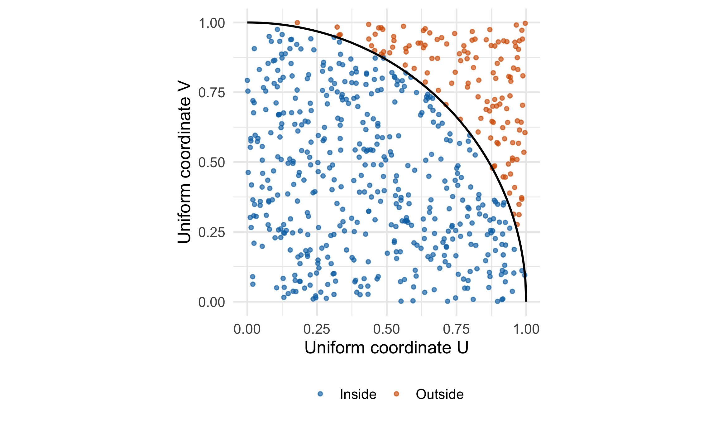

A quarter circle inside the unit square, with blue points inside and orange points outside. — Figure 5.3: Uniform points turn the area ratio into a success probability. The plotted points are a subset of the simulation; the estimate uses all 4,000 points.

Why multiply by 4? The proportion inside estimates \(\pi/4\). Multiplying by 4 gives an estimate of \(\pi\).

5.2.2 An integral is width times average height

For \(X\sim\operatorname{Uniform}(a,b)\),

\[ \int_a^b g(x)\,dx=(b-a)\mathbb{E}[g(X)]. \]

This gives a simple recipe: sample across the interval, average the function values, and multiply by the interval’s width.

For \(\int_2^4 e^{-x}\,dx\), the interval has width \(4-2=2\).

set.seed(8670)
N <- 10000
x <- runif(N, 2, 4)
y24 <- 2 * exp(-x)  # width times the function value
c(mean_height = mean(y24) / 2,
  estimate = mean(y24), exact = exp(-2) - exp(-4))
#> mean_height    estimate       exact 
#>  0.05805926  0.11611852  0.11701964

Code

height_grid <- data.frame(x = seq(2, 4, length.out = 301))
height_grid$height <- exp(-height_grid$x)
height_draws <- data.frame(x = x[1:40])
height_draws$height <- exp(-height_draws$x)
ggplot(height_grid, aes(x, height)) +
  geom_area(aes(fill = "Target integral (area under curve)"), alpha = .8) +
  geom_line(color = "black", linewidth = .8) +
  geom_segment(data = height_draws,
    aes(xend = x, y = 0, yend = height,
        color = "Sampled heights (first 40 draws)",
        linetype = "Sampled heights (first 40 draws)"), alpha = .4) +
  geom_hline(aes(yintercept = mean(y24) / 2,
                 color = "Mean height (all 10,000 draws)",
                 linetype = "Mean height (all 10,000 draws)"), linewidth = .8) +
  scale_color_manual(name = NULL,
    breaks = c("Sampled heights (first 40 draws)", "Mean height (all 10,000 draws)"),
    values = c("Sampled heights (first 40 draws)" = "#0072B2",
               "Mean height (all 10,000 draws)" = "#D55E00")) +
  scale_linetype_manual(name = NULL,
    breaks = c("Sampled heights (first 40 draws)", "Mean height (all 10,000 draws)"),
    values = c("Sampled heights (first 40 draws)" = "solid",
               "Mean height (all 10,000 draws)" = "dashed")) +
  scale_fill_manual(name = NULL,
    values = c("Target integral (area under curve)" = "#E6F2EC")) +
  guides(color = guide_legend(order = 1, ncol = 1,
                              override.aes = list(alpha = 1)),
         linetype = guide_legend(order = 1, ncol = 1),
         fill = guide_legend(order = 2,
                             override.aes = list(color = "#7DAF95", alpha = 1))) +
  labs(x = "x", y = "Integrand exp(-x)",
       subtitle = sprintf("Mean height = %.6f; integral estimate = %.6f",
                          mean(y24) / 2, mean(y24))) +
  theme(legend.position = "bottom", legend.box = "vertical",
        legend.text = element_text(size = 10),
        legend.key.width = grid::unit(1.3, "lines"),
        legend.key.height = grid::unit(.8, "lines"),
        legend.margin = margin(0, 0, 0, 0),
        legend.spacing.y = grid::unit(.1, "lines"))

The black curve is exp(-x) on 2 to 4. A legend identifies blue segments as sampled heights for the first 40 draws, the orange dashed line as the mean height of all 10,000 draws, and green shading as the target integral under the curve. The subtitle reports the same mean height and integral estimate as the code output. — Figure 5.4: The legend identifies sampled heights, their mean, and the target integral. Only the first 40 draws are shown; the orange mean uses all 10,000 draws. Multiplying this mean by width 2 gives the printed estimate of the shaded area.

This curve is the integrand, not a probability density on \([2,4]\). Its area is the integral we want; it need not equal 1.

Exercise 5.1 (In Class: Find the Missing Factor) A student uses mean(exp(-x)) to estimate \(\int_2^4 e^{-x}\,dx\). What factor is missing?

Solution 5.1. The width is 2. Use 2 * mean(exp(-x)), or average y24 <- 2 * exp(-x).

5.3 Monte Carlo Standard Error

Let \(X\sim P\) be the input and \(Y=g(X)\) the output. From \(N\) independent draws, estimate

\[ \theta=\mathbb{E}[g(X)],\qquad \widehat\theta=\overline Y=\frac1N\sum_{i=1}^N Y_i. \]

Our example uses \(X=U\sim\operatorname{Uniform}(0,1)\) and \(g(u)=e^u\), so \(\theta=e-1\).

Individual exp(U) values spread from 1 to e, while averages of 100 outputs cluster near e minus one. — Figure 5.5: Left: 400 individual outputs. Right: 400 independent runs, each averaging 100 outputs. The horizontal scale is the same; the dashed line marks e - 1.

Quantity	Meaning
\(s_X\)	Sample SD of inputs: `sd(x)` estimates \(\sqrt{\operatorname{Var}(X)}\).
\(\operatorname{Var}(Y)=\sigma_Y^2\)	Population variance of one output.
\(s_Y\)	Sample SD of outputs: `sd(y)` estimates \(\sigma_Y\); its square `var(y)` estimates \(\operatorname{Var}(Y)\).
MCSE	SD of the estimated mean \(\overline Y\) across runs.

For independent outputs with finite variance,

\[ \operatorname{MCSE}=\sqrt{\operatorname{Var}(\overline Y)} =\sqrt{\frac{\operatorname{Var}(Y)}{N}}, \qquad \widehat{\operatorname{MCSE}}=\frac{s_Y}{\sqrt N}. \]

To assess simulation precision, report the estimate and estimated MCSE. Use \(s_Y\) to describe individual outputs. Use \(s_X/\sqrt N\) only when averaging \(X\); here we average \(e^U\).

Specify the input distribution \(P\), output function \(g\), and sample size \(N\).
Draw \(X_1,\ldots,X_N\) independently from \(P\); compute \(Y_i=g(X_i)\).
Calculate \(\widehat\theta=\overline Y\) and the sample SD \(s_Y\) of these outputs.
Report \(\widehat\theta\) and estimated MCSE \(s_Y/\sqrt N\).

set.seed(8670)
N <- 10000
u <- runif(N)
y <- exp(u)
c(estimate = mean(y), s_X = sd(u), var_Y = var(y),
  s_Y = sd(y), MCSE = sd(y) / sqrt(N))
#>    estimate         s_X       var_Y         s_Y        MCSE 
#> 1.726713868 0.289668030 0.244172888 0.494138531 0.004941385

Here \(s_Y\approx0.494\) describes output spread; MCSE \(\approx0.00494\) describes precision of the mean. For large \(N\), an approximate 95% Monte Carlo interval is \(\overline Y\pm1.96\,\widehat{\operatorname{MCSE}}\). Four times as many draws halve MCSE; the population variance \(\operatorname{Var}(Y)\) stays unchanged.

5.4 Variance Reduction

Instead of increasing the sample size, we can change the values being averaged. If independent, identically distributed contributions \(W_1,\ldots,W_m\) satisfy \(\mathbb{E}[W_j]=\theta\), then

\[ \mathbb{E}[\overline W]=\theta, \qquad \operatorname{Var}(\overline W)=\frac{\operatorname{Var}(W)}{m}. \]

Variance reduction constructs contributions with less variance while retaining the same expectation. We will replace \(e^U\) by a pair average or an adjusted output. Since these constructions have different costs per contribution, we compare them at the same number of evaluations of exp().

5.5 Antithetic Variables

5.5.1 Why are both inputs uniform?

Let \(V=1-U\). Reflecting \([0,1]\) about its midpoint preserves interval lengths. More formally, for \(0\leq v\leq1\),

\[ P(V\leq v)=P(1-U\leq v)=P(U\geq1-v)=1-(1-v)=v. \]

Together with support \([0,1]\), this is the CDF of \(\operatorname{Uniform}(0,1)\). Thus \(U\) and \(V\) have the same distribution, but they are dependent: once \(U\) is known, \(V\) is determined.

5.5.2 What values do we average?

One uniform draw produces two outputs, \(Y_k=e^{U_k}\) and \(Y'_k=e^{1-U_k}\). First average within each pair, then average across pairs:

\[ A_k=\frac{e^{U_k}+e^{1-U_k}}{2},\qquad \widehat\theta_{\mathrm{anti}}=\frac1K\sum_{k=1}^K A_k. \]

For example, \(U_k=0.2\) gives outputs 1.2214 and 2.2255, hence \(A_k=1.7235\). The final estimate averages the \(K\) values \(A_1,\ldots,A_K\). Both outputs have mean \(\theta\), so \(\mathbb{E}[A_k]=(\theta+\theta)/2=\theta\).

As \(U\) increases, one output rises and the other falls. The figure shows how these fluctuations partly cancel.

The curves exp(U) and exp(1-U) slope in opposite directions; their pair average remains near the target. — Figure 5.6: The two outputs move in opposite directions. Their pair average is flatter, with the same mean e - 1 (dashed line).

5.5.3 Why does pairing reduce variance?

Write \(\sigma^2=\operatorname{Var}(Y)=\operatorname{Var}(Y')\) and \(\gamma=\operatorname{Cov}(Y,Y')\). Then

\[ \operatorname{Var}(A) =\frac14\{\sigma^2+\sigma^2+2\gamma\} =\frac{\sigma^2+\gamma}{2}. \]

Two independent outputs would give variance \(\sigma^2/2\) for their average. A negative covariance therefore helps. In this example, \(YY'=e^Ue^{1-U}=e\), so

\[ \gamma=\mathbb{E}[YY']-\mathbb{E}[Y]\mathbb{E}[Y'] =e-(e-1)^2\approx-0.2342<0. \]

With a budget of \(N=2K\) evaluations, the antithetic estimator has variance \((\sigma^2+\gamma)/(2K)\), compared with \(\sigma^2/(2K)\) for plain Monte Carlo. For a general function \(g\), reflection helps only if \(g(U)\) and \(g(1-U)\) have negative covariance; monotone \(g\) gives nonpositive covariance.

Choose \(K\) and \(T\) so \(T(X)\sim P\) when \(X\sim P\), and paired outputs have negative covariance.
Draw independent \(X_k\sim P\); evaluate \(Y_k=g(X_k)\) and \(Y_k^{\prime}=g(T(X_k))\).
Store \(A_k=(Y_k+Y_k^{\prime})/2\) for each pair.
Report \(\widehat\theta_{\mathrm{anti}}=K^{-1}\sum_{k=1}^K A_k\) and estimated MCSE \(s_A/\sqrt K\).

Here \(g(u)=e^u\) and \(T(u)=1-u\). Compute sd(pair_y) from the \(K\) independent pair averages. With \(K=5000\), the cost is 10,000 evaluations.

set.seed(8670)
K <- 5000
u <- runif(K)
pair_y <- (exp(u) + exp(1 - u)) / 2
c(estimate = mean(pair_y), MCSE = sd(pair_y) / sqrt(K))
#>     estimate         MCSE 
#> 1.7189273292 0.0008743739

5.6 Control Variates

A control variate \(C=h(X)\) has a known mean \(\mu_C\) and accompanies the output \(Y=g(X)\). Uppercase \(C\) is random; lowercase \(c\) is a fixed weight controlling the adjustment:

\[ Z=Y+c(C-\mu_C). \]

Since \(\mathbb{E}[C-\mu_C]=0\), \(\mathbb{E}[Z]=\theta\) for any fixed \(c\). Average the adjusted outputs:

\[ \widehat\theta_{\mathrm{cv}}=\overline Z =\overline Y+c(\overline C-\mu_C). \]

The difference \(\overline C-\mu_C\) measures how far this run’s control mean is from its known value.

5.6.1 How do we choose the coefficient?

Covariance measures joint variation:

\[ \operatorname{Cov}(C,Y)=\mathbb{E}[CY]-\mu_C\theta =\operatorname{Cov}(Y,C). \]

Positive covariance means \(C\) and \(Y\) tend to deviate from their means in the same direction; negative covariance means opposite directions. Choose \(c\) to minimize

\[ \operatorname{Var}(Z) =\operatorname{Var}(Y)+c^2\operatorname{Var}(C) +2c\operatorname{Cov}(C,Y). \]

Differentiate with respect to \(c\) and set the derivative to zero:

\[ 2c\operatorname{Var}(C)+2\operatorname{Cov}(C,Y)=0 \quad\Longrightarrow\quad c^*=-\frac{\operatorname{Cov}(C,Y)}{\operatorname{Var}(C)}. \]

For \(\operatorname{Var}(C)>0\), this is the minimum. The weight \(c^*\) has the opposite sign to the covariance: it cancels the variation in \(Y\) associated with \(C\). Zero covariance gives \(c^*=0\).

5.6.2 Calculate c for our example

Here \(g(u)=e^u\), \(h(u)=u\), \(\mu_C=1/2\), and \(\operatorname{Var}(C)=1/12\). Integration by parts gives

\[ \mathbb{E}[Ue^U]=\int_0^1 ue^u\,du =\left[(u-1)e^u\right]_0^1=1. \]

Therefore,

\[ \begin{aligned} \operatorname{Cov}(U,e^U) &=1-\frac{e-1}{2}\approx0.140859,\\ c^*&=-\frac{1-(e-1)/2}{1/12} =6e-18\approx-1.690309. \end{aligned} \]

The positive covariance gives \(c^*<0\): correct downward when \(U>0.5\) and upward when \(U<0.5\). For \(U=0.2\), \(Y\approx1.2214\) becomes \(Z\approx1.2214+(-1.6903)(0.2-0.5)=1.7285\).

The original curve rises steeply. Arrows move low-input outputs upward and high-input outputs downward to a flatter adjusted curve. — Figure 5.7: Arrows show the correction \(c^*(U - 0.5)\), with \(c^*=6e-18\approx-1.6903\). The adjusted curve is flatter; both curves have mean \(e-1\) (dashed line).

Choose \(N\), a control function \(h\) with known mean \(\mu_C=\mathbb{E}[h(X)]\), and a fixed coefficient \(c\) (ideally \(c^*\)).
Draw independent \(X_i\sim P\). From each input, calculate \(Y_i=g(X_i)\) and \(C_i=h(X_i)\).
Store \(Z_i=Y_i+c(C_i-\mu_C)\).
Report \(\widehat\theta_{\mathrm{cv}}=\overline Z\) and estimated MCSE \(s_Z/\sqrt N\), using the sample SD of the adjusted outputs.

set.seed(8670)
N <- 10000
u <- runif(N)
c_star <- -(1 - (exp(1) - 1) / 2) / (1 / 12)
adjusted_y <- exp(u) + c_star * (u - 0.5)
c(estimate = mean(adjusted_y), MCSE = sd(adjusted_y) / sqrt(N))
#>     estimate         MCSE 
#> 1.7187389937 0.0006251175

Use the known mean 0.5; substituting mean(u) makes the average adjustment zero. If the covariance is unknown, estimate \(c\) from independent pilot pairs with -cov(C, Y) / var(C), then hold it fixed for the main run.

5.7 Summary

Monte Carlo simulation shows what a specified probability model implies about uncertain outcomes. It can estimate average outputs, event probabilities, and integrals when direct calculation is difficult. In the shop example, average demand is 12, yet preparing 12 muffins leaves about a 42% chance of a shortage. Simulation quantifies that risk under the model’s assumptions.

The calculation depends on the question:

Expected output: simulate inputs and average their outputs \(g(X_i)\).
Event probability: average indicators, with 1 for an occurrence and 0 otherwise.
Integral over \([a,b]\): draw uniformly and average \((b-a)g(X_i)\).

Output variation describes differences among possible outcomes. MCSE describes uncertainty in the estimated average from a finite simulation. For independent contributions with finite variance, it decreases at rate \(1/\sqrt N\). More draws improve numerical precision; they do not remove real outcome variation or validate the model. A fixed seed reproduces a run but does not make it more accurate.

For \(\theta=\mathbb{E}[e^U]\), plain Monte Carlo averages the original outputs. Antithetic variables pair outputs whose fluctuations offset each other. Control variates use a correlated variable with a known mean to adjust each output. The latter two methods preserve the target while reducing the variance of the values being averaged.

Method	One value in the average	Estimate	MCSE
Plain MC	\(Y_i=e^{U_i}\)	\(\overline Y\)	\(s_Y/\sqrt N\)
Antithetic	\(A_k=(e^{U_k}+e^{1-U_k})/2\)	\(\overline A\)	\(s_A/\sqrt K\)
Control variate	\(Z_i=e^{U_i}+c^*(U_i-1/2)\)	\(\overline Z\)	\(s_Z/\sqrt N\)

Compare methods at the same computational cost. Here each uses 10,000 evaluations of exp(): \(N=10{,}000\) independent draws for plain MC and control variates, or \(K=5{,}000\) independent pairs for antithetic variables. Compare MCSE, since closeness to \(e-1\) in one run can be due to chance.

5.8 Supplementary

Optional reading; not on the exam:

Art B. Owen (2013), Monte Carlo Theory, Methods and Examples, available online. Read Chapter 2 for Monte Carlo estimation and error assessment; Chapter 8, Sections 8.2 and 8.9, for antithetic and control variates.
Christian P. Robert and George Casella (2010), Introducing Monte Carlo Methods with R. Chapters 3 and 4 cover Monte Carlo integration and methods for controlling and accelerating convergence, with R examples.
2025 course notes: variance and efficiency, antithetic variables, and control variates.
Detailed derivations, pilot estimation, and additional examples: the earlier version of this chapter, under Supplementary.