6 Cross Validation
Monte Carlo simulation generates inputs from a specified model. Cross-validation (CV) reuses observed data to ask a different question: how well will a fitting method predict new observations? We use CV to compare models and choose their complexity.
The main idea is fit on one part, predict the part left out, and average the prediction errors. We use one polynomial regression example throughout.
6.1 Prediction on New Observations
For regression, we want the average squared prediction error on independent new observations from the same population.
Training error uses the observations that fitted the model. It is usually optimistic: the model has already used their outcomes to choose its coefficients. To assess prediction, evaluate observations left out of fitting.
For \(m\) held-out observations, calculate
\[ \operatorname{MSE}=\frac1m\sum_{i=1}^m(y_i-\widehat y_i)^2. \]
For classification, we could instead average \(\mathbf{1}\{y_i\ne\widehat y_i\}\) to estimate the misclassification rate. Choose the loss before comparing models.
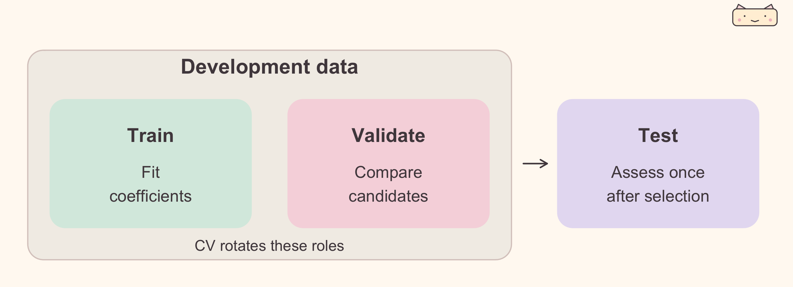
A single training/validation split is simple, but its result depends on which observations were held out. CV spreads validation across several subsets. A final test set remains separate from this model-selection process.
6.2 One Example: Choose a Polynomial Degree
We compare polynomial regressions
\[ \widehat f_d(x)=\widehat\beta_0+\widehat\beta_1x+\cdots+\widehat\beta_dx^d, \qquad d\in\{1,\ldots,8\}. \]
The degree \(d\) is a hyperparameter: it specifies the model’s flexibility. The coefficients \(\beta_0,\ldots,\beta_d\) are parameters estimated from training data after we fix \(d\). Hyperparameter tuning compares candidate settings using validation error. Here least squares estimates the coefficients; CV chooses the degree.
Other hyperparameters include the ridge penalty \(\lambda\) and the number of neighbors in \(k\)-nearest neighbors. The number of CV folds \(K\) controls the evaluation procedure, not the polynomial’s flexibility.
Generate one illustrative data set with a quadratic mean and random noise. Reserve 40 observations for the final test; use 80 for development. All observations are generated independently, so these disjoint groups are independent samples.
set.seed(8670)
x <- runif(120, -2, 2)
dat <- data.frame(x, y = 1 + 2 * x - x^2 + rnorm(120, sd = 0.7))
development <- dat[1:80, ]
test <- dat[81:120, ]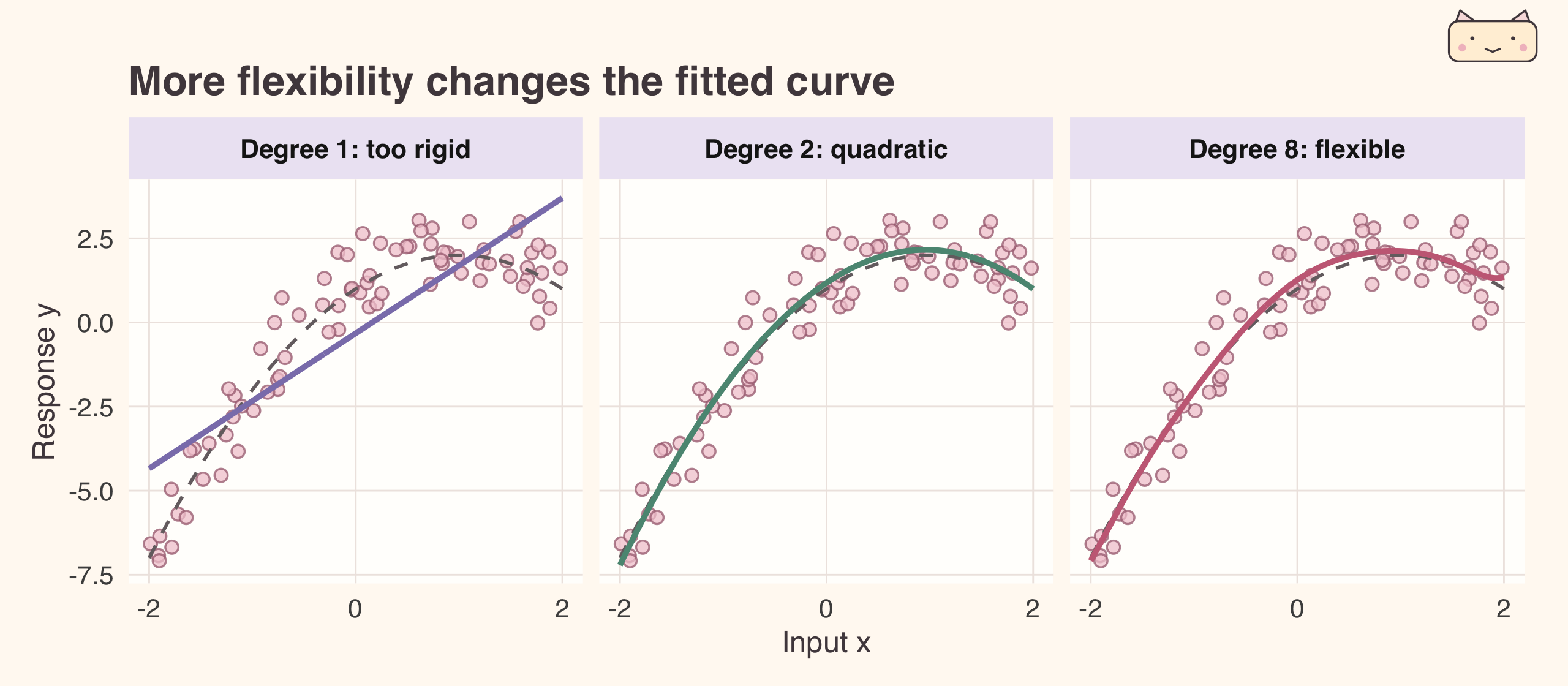
6.2.1 Underfitting and Overfitting
Underfitting: the model is too restrictive to capture the main pattern. A straight line misses the curvature here. Training and validation errors tend to be large relative to a suitable model. Increasing flexibility can help.
Overfitting: the model adapts to training-sample noise that does not generalize. A typical sign is training error falling while validation error increases. A high degree creates the possibility of overfitting; complexity alone does not prove it.
A rigid model can have high bias (systematically miss the mean pattern). A flexible model can have high variance (change substantially with another training sample). We want enough flexibility to learn the pattern without fitting too much noise.
For nested least-squares models, training MSE cannot increase when we add polynomial terms. Choosing by training MSE therefore favors the largest degree, even when prediction gets worse. CV compares held-out errors instead; see the error curves below.
6.3 How K-Fold CV Works
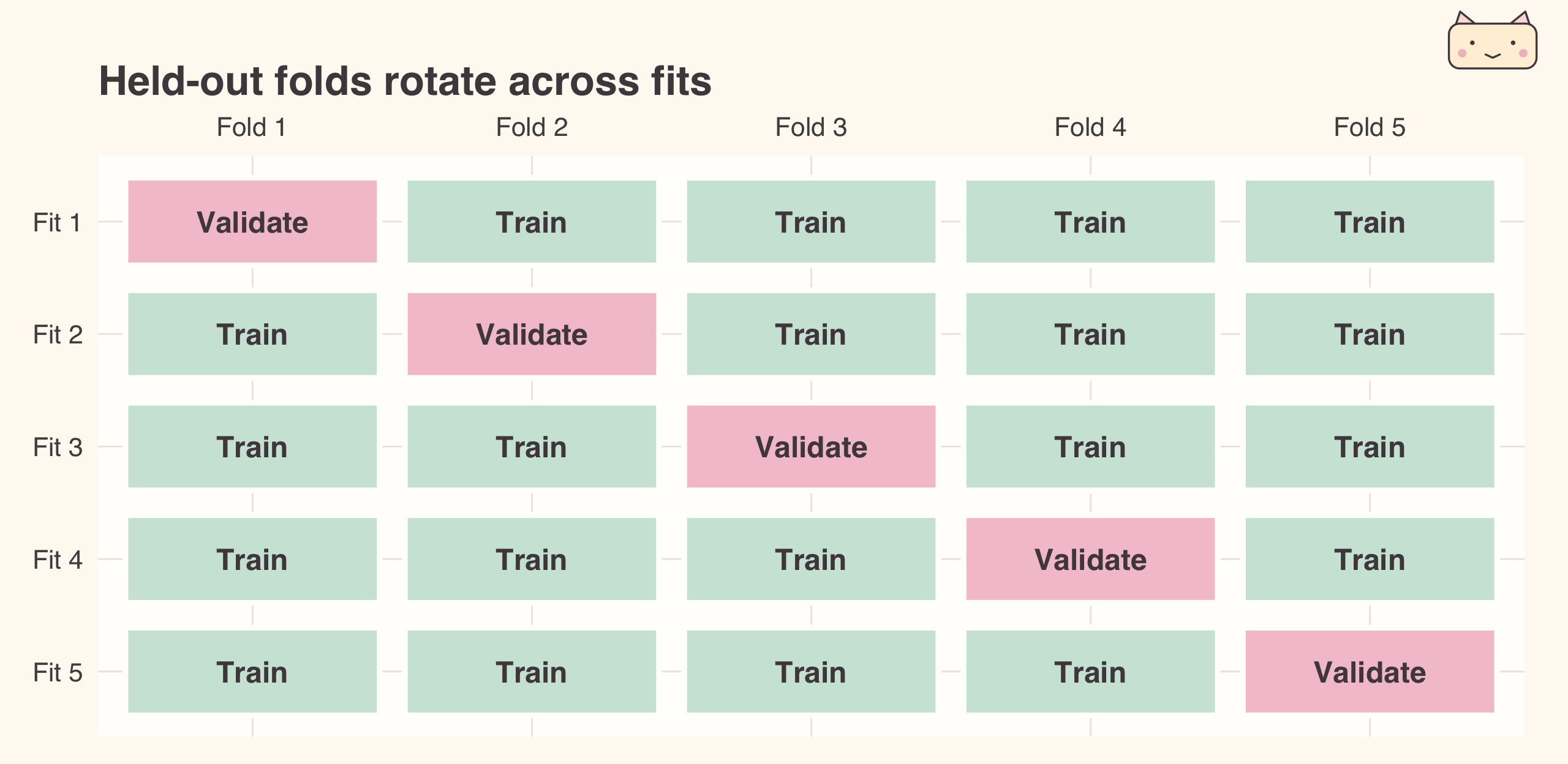
Split the \(n\) development observations into \(K\) roughly equal folds. Each fold serves once as validation data; the other \(K-1\) folds supply the training data. Every observation receives a prediction from a model fitted without that observation.
For one fixed degree, 5-fold CV means five separate fits. Keep the degree fixed but estimate new coefficients each time. Each observation is used for validation once and training four times; it never serves both roles in the same fit.
- Choose the candidate models and the loss. Randomly assign the development observations to \(K\) folds; use the same folds for every candidate.
- For each candidate, and for each fold \(k\), fit a fresh model on all folds except \(k\).
- Predict the outcomes in fold \(k\) and store their losses. Repeat until every observation has one held-out prediction.
- Average all \(n\) held-out losses to obtain that candidate’s CV error. Select the candidate with the smallest error.
Let \(S_k\) contain the indices in fold \(k\), and let \(\widehat f_d^{(-k)}\) be the degree-\(d\) model fitted without that fold. Then
\[ \operatorname{CV}(d) =\frac1n\sum_{k=1}^K\sum_{i\in S_k} \left(y_i-\widehat f_d^{(-k)}(x_i)\right)^2. \]
What is averaged? The squared errors of the held-out predictions. If a held-out outcome is 3 and its prediction is 2.5, it contributes \((3-2.5)^2=0.25\). With \(n=80\), sum all 80 such errors and divide by 80. Equal-sized folds also allow averaging their MSEs; unequal folds require weights \(|S_k|/n\).
6.4 Leave-One-Out CV (LOOCV)
LOOCV is \(K=n\): each validation fold contains one observation. For a fixed degree \(d\), our 80 development observations give:
| Fit | Training observations | Held-out prediction |
|---|---|---|
| 1 | All except observation 1 | Predict \(y_1\) from \(x_1\) |
| 2 | All except observation 2 | Predict \(y_2\) from \(x_2\) |
| \(\vdots\) | \(\vdots\) | \(\vdots\) |
| 80 | All except observation 80 | Predict \(y_{80}\) from \(x_{80}\) |
Write \(\widehat f_d^{(-i)}\) for the model refitted without observation \(i\). Average its \(n\) held-out squared errors:
\[ \operatorname{CV}_{\mathrm{LOO}}(d) =\frac1n\sum_{i=1}^n \left(y_i-\widehat f_d^{(-i)}(x_i)\right)^2. \]
Each fit supplies one squared error, not a useful error estimate by itself. Predicting all observations with a model fitted to all \(n\) would give training error, not LOOCV. Repeat the leave-one-out procedure for each candidate degree.
LOOCV trains on almost all the data but usually costs more: 80 fits per degree here, versus 5 for 5-fold CV. For a deterministic fitting method, LOOCV has no random fold assignment. Its score still varies across new data sets; it is not automatically more accurate or less variable than 5-fold CV.
6.5 Select, Refit, and Test
Now tune \(d\) using 5-fold CV: the outer loop tries degrees \(1,\ldots,8\); the inner loop computes a CV score for one fixed degree. Choose
\[ d^*=\arg\min_{d\in\{1,\ldots,8\}}\operatorname{CV}(d). \]
prediction[fold == k] stores the held-out predictions. poly(x, d) uses a numerically stable basis for a degree-\(d\) polynomial.
K <- 5
fold <- sample(rep(1:K, length.out = nrow(development)))
degrees <- 1:8
cv_mse <- numeric(length(degrees))
for (d in degrees) {
  prediction <- numeric(nrow(development))
  for (k in 1:K) {
    fit <- lm(y ~ poly(x, d), data = development[fold != k, ])
    prediction[fold == k] <- predict(fit, development[fold == k, ])
  }
  cv_mse[d] <- mean((development$y - prediction)^2)
}
best_degree <- degrees[which.min(cv_mse)]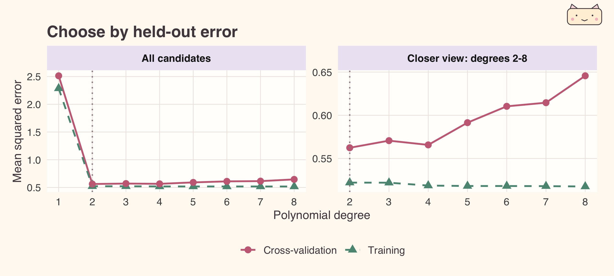
CV selects degree 2, with MSE 0.562. We now refit that degree on all 80 development observations, then use the 40 reserved test observations once:
final_fit <- lm(y ~ poly(x, best_degree), data = development)
test_prediction <- predict(final_fit, newdata = test)
c(degree = best_degree, test_MSE = mean((test$y - test_prediction)^2))
#>   degree test_MSE
#> 2.000000 0.413982
The final model is a new fit on all development data, not the best-scoring fold’s model. We use \(8\times5=40\) CV fits and one final fit. We average held-out losses to choose the degree, not the five fitted models.
The test MSE estimates prediction error for this final fit. It need not equal the CV MSE: CV used smaller training sets and different held-out observations. The minimum CV error can also be optimistic because we selected it from several candidates. If test error makes us change the degree, that set has become another validation set. Keep it out of model selection.
6.6 Choose Folds and Avoid Leakage
5-fold or 10-fold CV is a useful starting point for independent observations. Each fit uses a fraction \((K-1)/K\) of the development data: with \(n=80\), that means 64 training observations for 5-fold, 72 for 10-fold, and 79 for LOOCV.
Larger \(K\) reduces the training-size difference from the final fit but requires more fits. This training-size issue is different from model bias due to underfitting. Increasing \(K\) does not automatically improve the model or make CV less variable. A repeated-CV illustration is in Supplementary.
Two practical details determine whether the comparison is fair:
- Fit the whole procedure inside each training fold. Learn imputation, scaling, or feature selection using that fold’s training observations, then apply those choices to its validation observations. Using validation outcomes to select features before CV leaks information.
- Split according to the prediction task. Keep repeated observations from the same person together when predicting new people. For future prediction, train on the past and validate on later times; randomly shuffling time points can use future information.
6.7 Summary
Cross-validation estimates how a fitting procedure predicts observations excluded from training. It helps choose a model or hyperparameter when the population prediction error cannot be calculated directly. Its score measures predictive performance for the chosen loss and a comparable population; it does not establish that the model is the true data-generating mechanism.
The workflow is: define the prediction task and loss, hold out a test set, compare candidates by CV, refit the selected candidate, and assess it on the test set. Use the same folds for all candidates, and keep all data-dependent fitting inside the training folds.
| Method | Training / validation per fit | Fits per candidate | Main consideration |
|---|---|---|---|
| One split | One training set / one holdout | 1 | Fast; sensitive to the split |
| \(K\)-fold CV | \(K-1\) folds / one fold | \(K\) | Every observation is held out once |
| LOOCV | \(n-1\) observations / one | \(n\) | Nearly full training size; often costly |
| Repeated \(K\)-fold (optional) | Repeat the fold assignment | \(RK\) | Checks sensitivity to partitioning |
Here \(n\) is the development sample size and \(R\) is the number of repetitions. The separate final test set is not one of the CV folds.
6.8 Supplementary
Optional reading:
- James, Witten, Hastie, and Tibshirani (2021), An Introduction to Statistical Learning, 2nd edition. Chapter 5, especially Section 5.1 and the R lab, develops validation, LOOCV, and \(K\)-fold CV.
- Hastie, Tibshirani, and Friedman (2009), The Elements of Statistical Learning, 2nd edition. Sections 7.2-7.3 discuss bias and variance; Section 7.10 covers CV and why every model-building step belongs inside validation.
- 2025 STAT 8670 lecture: additional models and the ironslag example.
6.8.1 Repeated CV (optional)
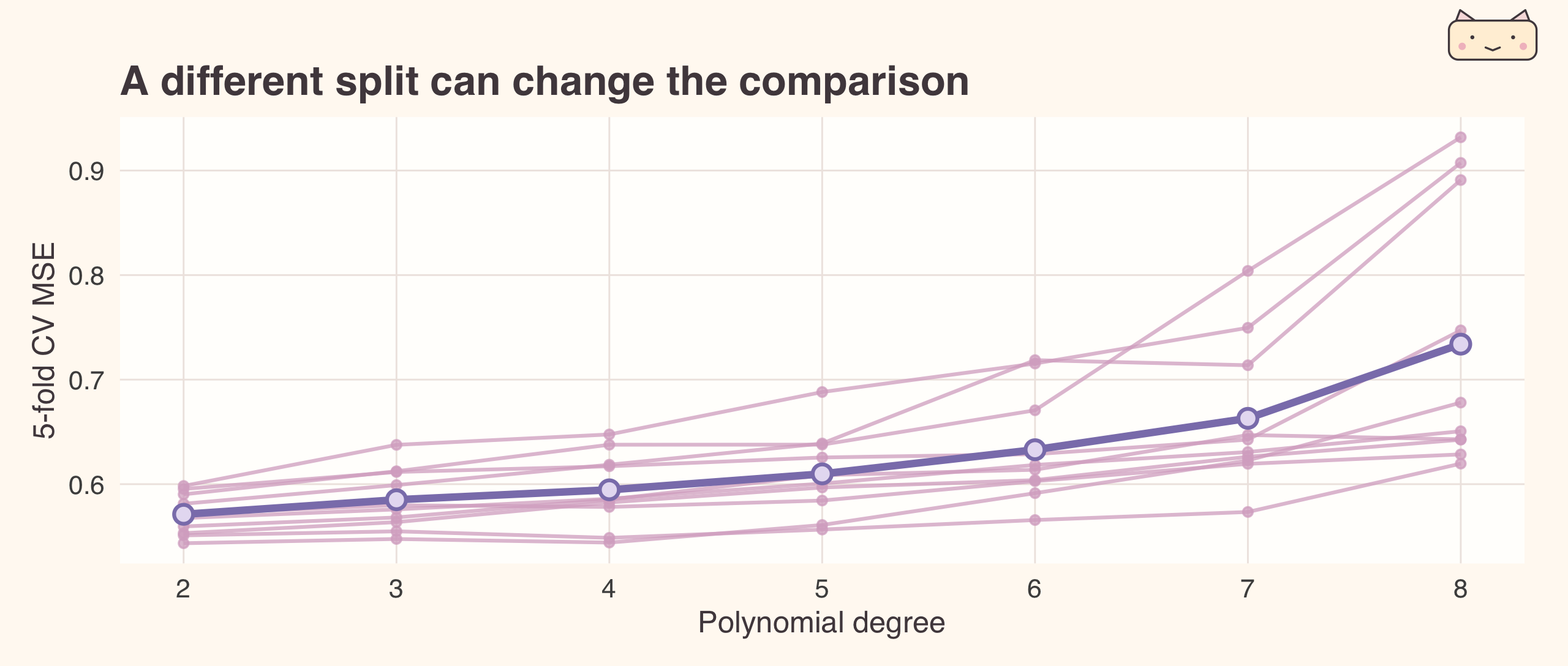
Repeating CV checks sensitivity to the fold assignment; it does not create new observations. Here several degrees have similar scores. A tiny improvement in one partition is weak evidence for a more complex model. The repeated curves describe split sensitivity, not independent experiments or a confidence interval.