7 Jackknife and Bootstrap
7.1 Introduction
This chapter continues from the previous chapter, introducing more resampling methods: jackknife and bootstrap techniques. We use the observed sample to assess the accuracy of an estimator when the population distribution is unknown or a formula is difficult to obtain.
We use one biomedical example throughout. The core lesson covers the concepts, algorithms, SE and bias estimates, and a bootstrap percentile interval. Longer derivations and other interval methods are in Supplementary.
Most of the methods follow Chapter 8 of Rizzo, M. L. (2007), Statistical Computing with R. CRC Press.
7.2 Resampling Methods
Resampling methods use the observed data to generate hypothetical samples. In the nonparametric bootstrap, we treat the observed sample as a finite population and draw random samples from it to make inferences about the population that was sampled. Resampling is useful when:
- We do not know the underlying population distribution.
- A formula for the uncertainty of an estimator is difficult to calculate.
Some commonly used resampling methods include:
- Cross-validation: assess how accurately a predictive model will perform on new data; see Chapter 6.
- Bootstrap: sample with replacement to estimate an estimator’s sampling distribution, SE, and bias.
- Jackknife: leave one observation out at a time to estimate SE and bias and examine sensitivity to individual observations.
- Permutation tests: rearrange labels in a way justified under a null hypothesis to construct a reference distribution for testing.
This chapter focuses on bootstrap and jackknife for uncertainty in an estimated parameter.
7.3 Estimators
Let \(D=(X_1,\ldots,X_n)\) be an independent sample from a population distribution \(F\). A parameter \(\theta\) describes the population; an estimator \(\hat\theta=T(D)\) is a rule calculated from the sample. Once we observe \(D\), it gives one numerical estimate.
The sampling distribution is the distribution of \(\hat\theta\) across repeated samples of size \(n\) from \(F\).
\[ \operatorname{SE}(\hat\theta)=\sqrt{\operatorname{Var}_F(\hat\theta)}, \qquad \operatorname{Bias}(\hat\theta)=\mathbb E_F(\hat\theta)-\theta. \]
SE measures spread; bias measures average displacement from the true parameter. Both concern repeated samples, not the spread of the individual observations.
7.3.1 Bias–Variance Tradeoff of an Estimator
For most of the course, we have focused on unbiased estimators and compared their variances. An estimator with some bias may nevertheless have a smaller mean squared error.
For an estimator with finite second moment, \[ \operatorname{MSE}_F(\hat\theta) =\mathbb E_F[(\hat\theta-\theta)^2] =\operatorname{Var}_F(\hat\theta)+\{\operatorname{Bias}_F(\hat\theta)\}^2. \]
Question: Why do we care about bias? Subtracting an estimated bias can also change variance, so a bias-corrected estimator need not have smaller MSE. The derivation is in Supplementary.
7.4 Bootstrap
Bootstrap estimates of a sampling distribution are analogous to the idea of density estimation. A histogram estimates a density’s shape; it is not the density itself. In the same spirit, the bootstrap uses the empirical distribution of a sample in place of the unknown population distribution.
Suppose we have an observed random sample \(x=(x_1,\ldots,x_n)\) from \(F\). Generate an index \(I\) uniformly from \(\{1,\ldots,n\}\) and select \(X^*=x_I\). Each row index has probability \(1/n\). If a value occurs more than once, its probability is its relative frequency in the sample.
Resampling generates \(X_1^*,\ldots,X_n^*\) by sampling with replacement. Conditional on the observed data, these draws are independent and have the empirical distribution \(F_n\).
7.4.1 Underlying, Sampling, and Bootstrap Distributions
- Underlying distribution \(F\): \(F(t)=P(X\le t)\) describes one observation from the population.
- Empirical distribution \(F_n\): \(F_n(t)=n^{-1}\sum_{i=1}^n\mathbf 1\{x_i\le t\}\) puts mass \(1/n\) on each observed value. It estimates \(F\) from one fixed sample.
- Sampling distribution \(G_n\): \(G_n(t)=P_F(T(D)\le t)\) describes a statistic across fresh samples of size \(n\) from \(F\). Its SD is the estimator’s SE.
- Bootstrap distribution \(F_n^*\): in this chapter, \(F_n^*(t)=P_*(T(D^*)\le t\mid D)\) describes the same statistic, conditional on the fixed sample \(D\). Draw each resample from \(F_n\); its centred distribution approximates the centred sampling distribution under suitable regularity conditions.
\(F\) and \(F_n\) describe data values; \(G_n\) and \(F_n^*\) describe statistics. Population sampling changes \(D\); bootstrap sampling fixes \(D\) and changes \(D^*\).
The two sampling paths are \[ \begin{aligned} F &\longrightarrow D=(X_1,\ldots,X_n) \longrightarrow \hat\theta=T(D),\\ F_n &\longrightarrow D^*=(X_1^*,\ldots,X_n^*) \longrightarrow \hat\theta^*=T(D^*). \end{aligned} \]
Repeat the first path with new data to obtain the sampling distribution \(G_n\); repeat the second path with \(D\) fixed to obtain \(F_n^*\). The bootstrap uses the conditional distribution of \(\hat\theta^*-\hat\theta\) to approximate the sampling distribution of \(\hat\theta-\theta\); the two raw distributions need not have the same centre.
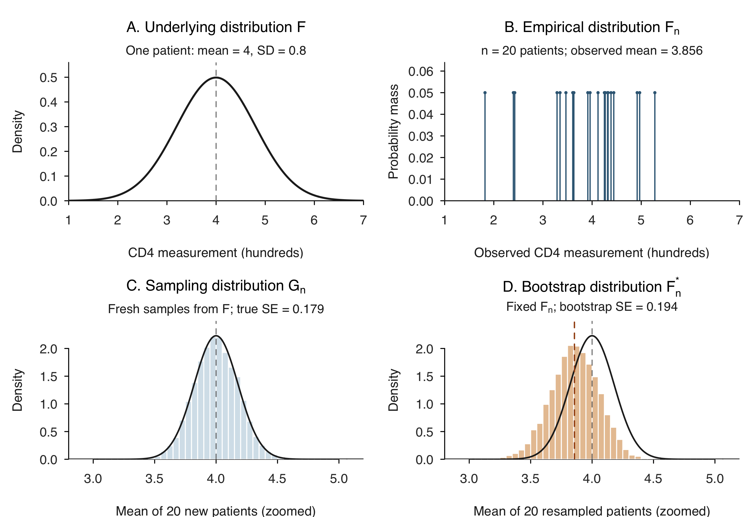
Biomedical illustration: follow the sampling process.
For this illustration only, suppose a patient’s CD4 measurement (in hundreds) follows the hypothetical population model \(X\sim N(4,0.8^2)\). Estimate the population mean using \(n=20\) independent patients. This model is chosen to make the distributions transparent; it is not fitted to the clinical dataset used below.
The figure follows two experiments. Population sampling: repeatedly draw 20 new patients from \(F\) and calculate a mean, giving \(G_n\). Bootstrap sampling: draw one sample once to obtain \(F_n\), keep it fixed, and resample 20 rows with replacement to calculate each mean, giving \(F_n^*\). Both use the same sample size and statistic.
In A, the random quantity is one patient’s measurement. In C and D, it is a mean of 20 measurements. The exact sampling distribution is \(\bar X\sim N(4,0.8^2/20)\), so its SE is \(0.8/\sqrt{20}\approx0.179\). The bootstrap distribution is centred at the observed mean, 3.856, not necessarily the true mean 4. Its different centre and spread arise from the particular sample in B.
Panel B is \(F_n\), not the sampling distribution: it has one mass \(1/20\) at each observed value. Panel D estimates \(F_n^*\) using means of whole resamples from B. Increasing \(B\) reduces Monte Carlo noise; it does not change \(F_n\) or force \(F_n^*\) to equal \(G_n\). The near-normal shape here is a feature of this example, not a requirement for bootstrap.
There are two approximations: replacing \(F\) by \(F_n\), and using finitely many bootstrap statistics to approximate \(F_n^*\). Increasing \(B\) improves only the second approximation.
7.4.2 Clinical Example: CD4 Measurements Before and After Treatment
For real clinical data, \(F\) and the true sampling distribution are unknown. We now use a biomedical dataset and keep the same resampling logic, changing the statistic from a mean to a correlation.
The dataset boot::cd4 contains 20 HIV-positive patients with CD4 measurements at baseline and after one year of antiviral treatment. Both columns are recorded in hundreds. Each row is one patient, with that patient’s two measurements kept together. We use independent patients as the sampling units.
Our parameter is \(\theta=\operatorname{Corr}(\mathrm{baseline},\mathrm{oneyear})\) in the population represented by these patients. We estimate it by the sample correlation.
Question: How uncertain is the association between patients’ baseline and one-year CD4 measurements?
See the official CD4 dataset documentation. This correlation describes association; it does not measure the treatment’s causal effect.
Show R code
data(cd4, package = "boot")
n <- nrow(cd4)
theta_hat <- cor(cd4$baseline, cd4$oneyear)
head(cd4, 3)
#>   baseline oneyear
#> 1     2.12    2.47
#> 2     4.35    4.61
#> 3     3.39    5.26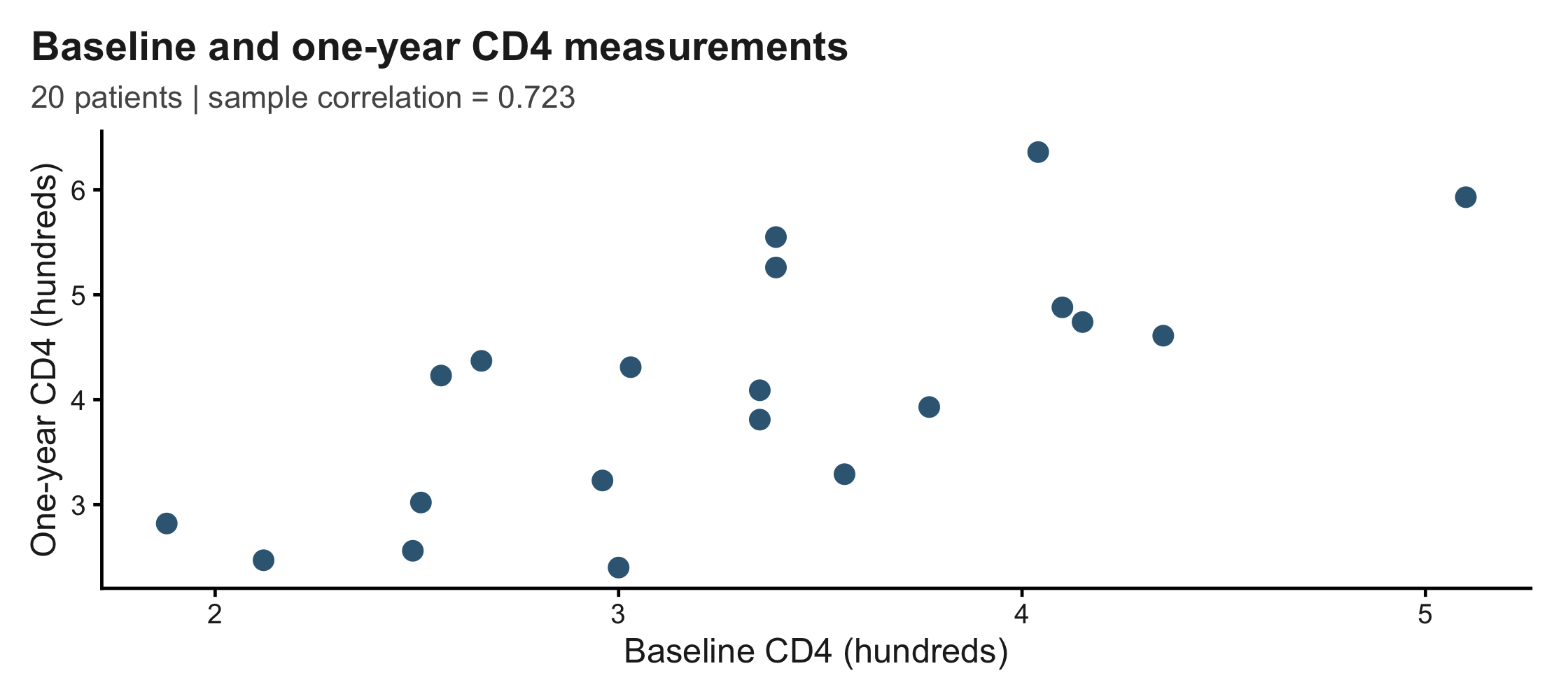
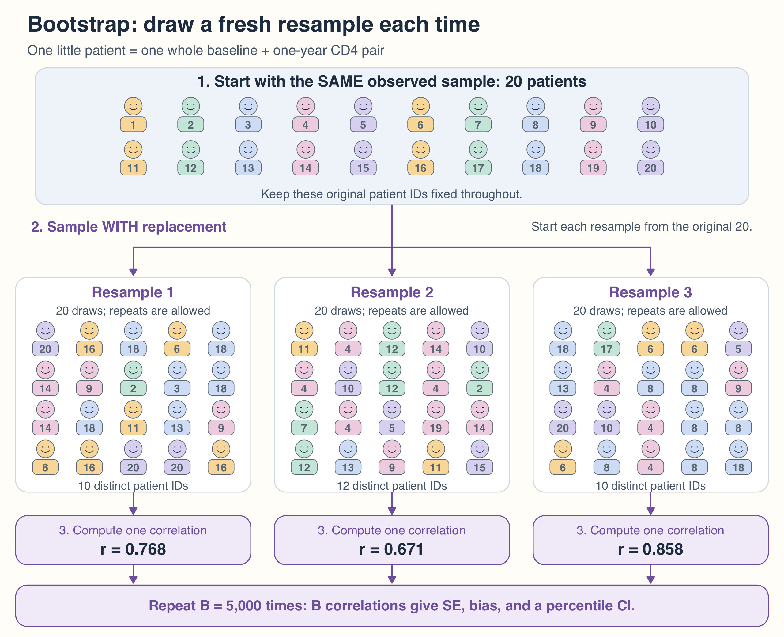
Think of putting the 20 patient IDs into a bag. Draw one ID, record that patient’s entire baseline/one-year CD4 row, return the ID to the bag, and repeat until you have 20 rows. Some patients appear more than once; others are absent. Compute one correlation, then repeat the whole process.
Input: \(n\) independent observations \(D\), a statistic \(T\), and a number of resamples \(B\).
- Calculate the observed estimate \(\hat\theta=T(D)\).
- For each \(b=1,\ldots,B\):
- Draw \(n\) row indices independently and uniformly from \(\{1,\ldots,n\}\), with replacement.
- Take those whole rows as one bootstrap sample \(D^{*(b)}\).
- Calculate one statistic \(\hat\theta^{*(b)}=T(D^{*(b)})\).
- Return the \(B\) statistics. Use their SD to estimate SE, their mean minus \(\hat\theta\) to estimate bias, and their quantiles for a percentile interval, as shown below.
Output: the empirical distribution of \(\hat\theta^{*(1)},\ldots,\hat\theta^{*(B)}\), which approximates the conditional bootstrap distribution \(F_n^*\) of the statistic.
As in Figure 7.1, \(F_n\) supplies individual observations, while the bootstrap distribution contains statistics. Here each statistic is a correlation of 20 paired measurements, rather than a mean of 20 values.
7.4.3 Apply the Algorithm to the CD4 Data
Show R code
# Seed once, then continue the random-number stream across all B resamples.
set.seed(8670)
B <- 5000
boot_theta <- numeric(B)
first_indices <- matrix(NA_integer_, nrow = n, ncol = 3)
for (b in seq_len(B)) {
  i <- sample.int(n, size = n, replace = TRUE)
  boot_theta[b] <- cor(cd4$baseline[i], cd4$oneyear[i])
  if (b <= 3) first_indices[, b] <- i
}
WarningResample whole rows, with replacement
Without replacement: drawing all 20 rows only rearranges the same data, so every correlation equals 0.723 and the estimated SE is zero.
Separate column resampling: drawing baseline and one-year CD4 measurements independently breaks the observed pairing and destroys the association we want to study.
7.4.4 Bootstrap Estimation of Standard Error
Recall that a normal-approximation interval for a population mean has the form \[\bar x\pm z_{1-\alpha/2}\frac{\sigma}{\sqrt n}.\] Here \(\sigma/\sqrt n\) is the standard error, while \(z_{1-\alpha/2}\sigma/\sqrt n\) is the margin of error. For a more complicated statistic, the bootstrap estimates SE from its replicates.
Let \(\bar\theta^*=B^{-1}\sum_{b=1}^B\hat\theta^{*(b)}\). The bootstrap estimate of the standard error of \(\hat\theta\) is the sample SD of the replicates: \[ \widehat{\operatorname{SE}}_{\mathrm{boot}}(\hat\theta) =\sqrt{\frac1{B-1}\sum_{b=1}^B(\hat\theta^{*(b)}-\bar\theta^*)^2}. \]
Show R code
boot_se <- sd(boot_theta)
boot_se
#> [1] 0.09042147
For the CD4 correlation, the estimated SE is 0.0904. Do not divide it by \(\sqrt B\): that would estimate the Monte Carlo error of the bootstrap mean, not the sampling uncertainty of \(\hat\theta\). We use \(B=5000\) here to obtain stable SE and percentile estimates; more resamples do not add patients.
7.4.5 Bootstrap Estimation of Bias
Recall that the bias of an estimator is \(\operatorname{Bias}_F(\hat\theta)=\mathbb E_F[\hat\theta]-\theta\). The bootstrap uses the same idea under \(F_n\). For a plug-in statistic such as our correlation, the original estimate \(\hat\theta\) plays the population-parameter role, and the average of the bootstrap statistics estimates their conditional expectation.
\[ \widehat{\operatorname{bias}}_{\mathrm{boot}} =\bar\theta^*-\hat\theta, \qquad \bar\theta^*=\frac1B\sum_{b=1}^B\hat\theta^{*(b)}. \]
Positive estimated bias suggests overestimation on average; negative estimated bias suggests underestimation. If bias correction is wanted, use \(\hat\theta_{\mathrm{boot,bc}}=\hat\theta-\widehat{\operatorname{bias}}_{\mathrm{boot}}\).
Show R code
boot_bias <- mean(boot_theta) - theta_hat
boot_bias
#> [1] -0.006977374
The estimated bias is -0.0070, small relative to the estimated SE. This alone is not a reason to replace the observed correlation with a bias-corrected estimate.
7.5 Jackknife
The jackknife is another resampling technique used to estimate the bias and variance of a statistic. It uses the same deletion operation as leave-one-out cross-validation, but here we calculate a parameter estimate from each retained sample rather than a prediction error.
Remove observation \(i\) to obtain \(D_{(-i)}\). The jackknife replicate is \(\hat\theta_{(-i)}=T(D_{(-i)})\), the same statistic calculated from the remaining \(n-1\) observations.
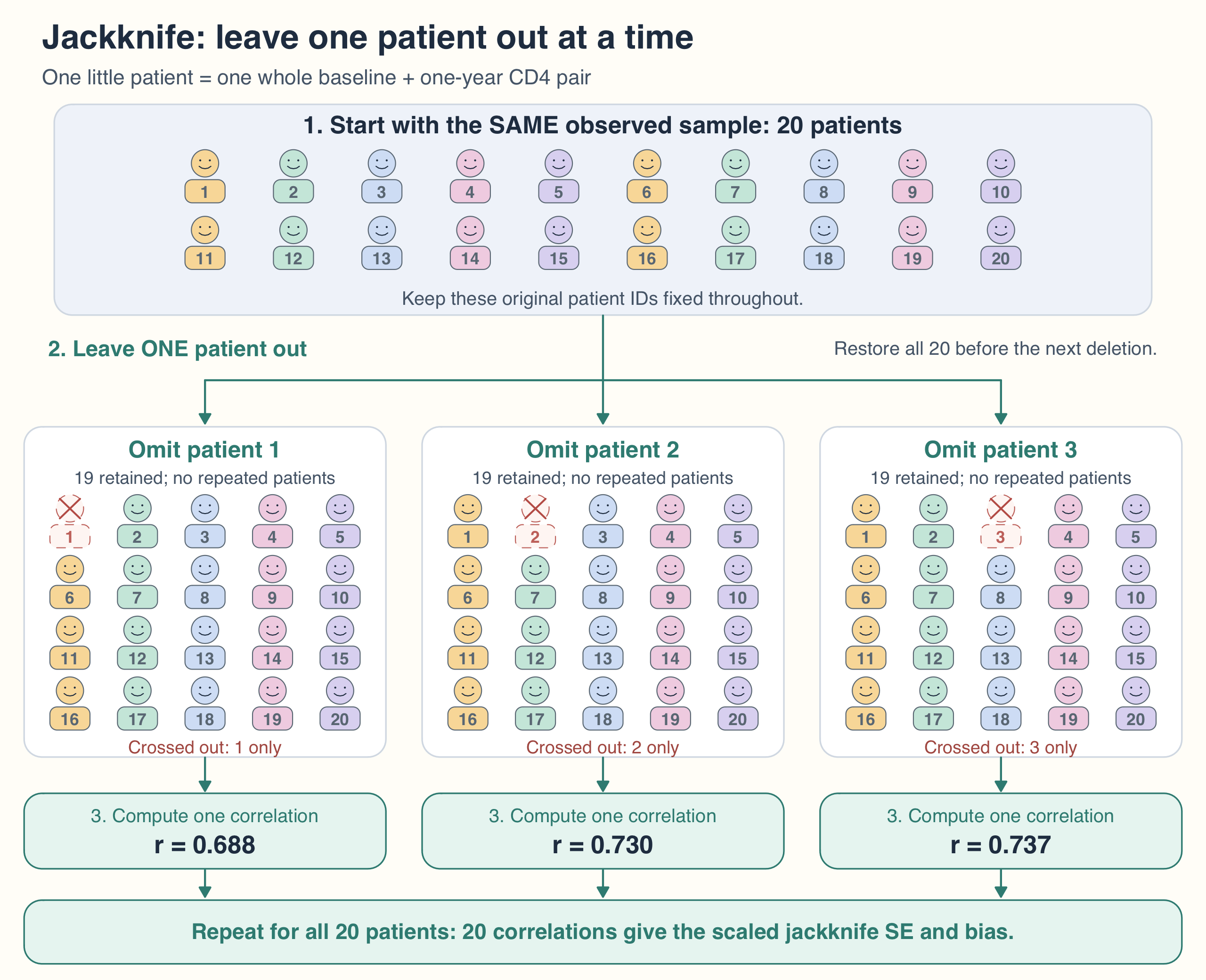
There are exactly \(n\) delete-one samples. Every observation is omitted once; no random sampling is needed. The changes in the statistic measure its sensitivity to individual observations.
For our correlation, \(n=20\) gives 20 replicates, each based on 19 patients. Figure 7.4 follows the first three deletions.
7.5.1 Jackknife Estimate of Bias
Let \(\bar\theta_{(-\cdot)}=n^{-1}\sum_{i=1}^n\hat\theta_{(-i)}\) be the average of the leave-one-out estimates. For a suitably smooth statistic, the jackknife estimates bias by
\[ \widehat{\operatorname{bias}}_{\mathrm{jack}} =(n-1)(\bar\theta_{(-\cdot)}-\hat\theta). \]
The bias-corrected estimate is \(\hat\theta_{\mathrm{jack,bc}}=\hat\theta-\widehat{\operatorname{bias}}_{\mathrm{jack}}\).
7.5.2 Jackknife Estimate of Standard Error
\[ \widehat{\operatorname{SE}}_{\mathrm{jack}}(\hat\theta) =\sqrt{\frac{n-1}{n}\sum_{i=1}^n (\hat\theta_{(-i)}-\bar\theta_{(-\cdot)})^2}. \]
Input: \(n\) independent observations \(D\) and a statistic \(T\).
- Calculate the full-sample estimate \(\hat\theta=T(D)\).
- For each \(i=1,\ldots,n\), delete row \(i\) and calculate \(\hat\theta_{(-i)}=T(D_{(-i)})\).
- Calculate the mean \(\bar\theta_{(-\cdot)}\) of the \(n\) replicates.
- Return the bias and SE estimates using the formulas above.
7.5.3 Apply the Algorithm to the Patients
Show R code
jack_theta <- numeric(n)
for (i in seq_len(n)) {
  jack_theta[i] <- cor(cd4$baseline[-i], cd4$oneyear[-i])
}| Patient omitted | Patients retained | Correlation | Change from full sample |
|---|---|---|---|
| 1 | 19 | 0.6884 | -0.0348 |
| 2 | 19 | 0.7302 | 0.0071 |
| 3 | 19 | 0.7374 | 0.0143 |
For example, omitting patient 1 changes the correlation from 0.723 to 0.688. This shows sensitivity to that observation; it does not establish that the patient is invalid or should be discarded. Use all 20 delete-one estimates for the following calculations.
NoteWhy not use the raw SD of the jackknife replicates?
The delete-one datasets overlap almost completely. Their raw SD measures the size of these small deletion changes; it is not the sampling SE of the full-sample estimator. With R’s sample-SD convention, the formula above equals
\[ \widehat{\operatorname{SE}}_{\mathrm{jack}} =\frac{n-1}{\sqrt n}\,\operatorname{sd}(\hat\theta_{(-1)},\ldots,\hat\theta_{(-n)}). \]
For the sample mean, this scaling gives exactly \(s/\sqrt n\). The bias factor \(n-1\) converts the small change from sample size \(n\) to \(n-1\) into an estimate of the leading bias at size \(n\). The derivations are in Supplementary.
Show R code
jack_mean <- mean(jack_theta)
jack_se <- sqrt((n - 1) / n * sum((jack_theta - jack_mean)^2))
jack_bias <- (n - 1) * (jack_mean - theta_hat)
jack_corrected <- theta_hat - jack_bias| Summary | Value |
|---|---|
| Mean of delete-one estimates | 0.7228 |
| Raw SD of delete-one estimates | 0.0213 |
| Jackknife SE | 0.0905 |
| Estimated bias | -0.0068 |
| Bias-corrected estimate | 0.7299 |
Here the raw SD is 0.0213, but the jackknife SE is 0.0905. The estimated bias is -0.0068; subtracting it gives the bias-corrected estimate 0.7299. The bias estimate is small relative to the SE, so this calculation alone is not a reason to replace the original estimate.
7.5.4 Jackknife Does Not Always Work
The delete-one jackknife works best for smooth statistics such as a mean or correlation. A non-smooth statistic such as a sample median can give unrepresentative delete-one changes, so the usual jackknife variance formula need not be consistent. Resampling is not a universal substitute for checking the statistic and sampling design.
7.6 Bootstrap Confidence Interval
Bootstrap replicates also give approximate confidence intervals for the target parameter. The 2025 notes introduce standard normal, basic, percentile, and bootstrap \(t\) intervals. We focus on the percentile interval in the core lesson; the other methods appear in Supplementary.
7.6.1 Bootstrap Percentile CI
Input: the \(B\) bootstrap statistics and a confidence level \(1-\alpha\).
- Find their empirical quantiles \(q^*_{\alpha/2}\) and \(q^*_{1-\alpha/2}\).
- Return the approximate \(100(1-\alpha)\%\) interval
\[ \mathrm{CI}_{\mathrm{perc}}= \left[q^*_{\alpha/2},\ q^*_{1-\alpha/2}\right]. \]
For 95% confidence, use the 2.5th and 97.5th percentiles of the statistics, not percentiles of the original observations.
Show R code
percentile_ci <- quantile(boot_theta, c(.025, .975))
percentile_ci
#>      2.5%     97.5%
#> 0.5071812 0.8586489
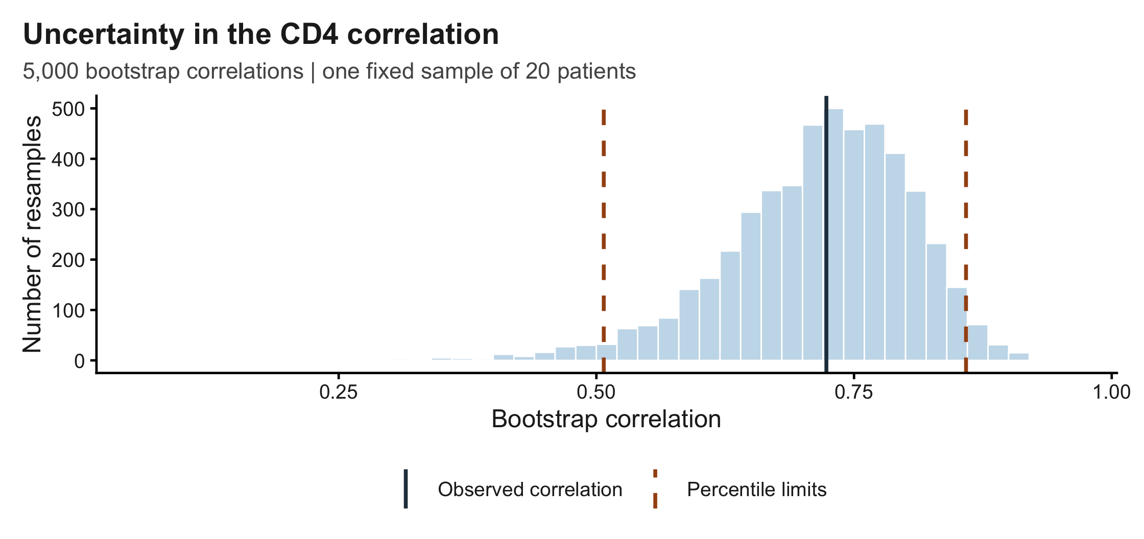
For these data, the nominal 95% percentile interval is [0.507, 0.859]. It follows the asymmetry of the bootstrap distribution instead of forcing equal distances on each side of \(\hat\theta\).
NoteInterpretation
The data suggest a positive association between patients’ baseline and one-year CD4 measurements, with substantial uncertainty about its magnitude. A nominal 95% confidence procedure aims for about 95% coverage across repeated original samples. This interval is approximate, especially with only 20 patients; it is not a 95% probability statement about the fixed parameter, a prediction interval for a new CD4 measurement, or a causal conclusion.
7.7 Summary and Practical Choices
Both methods assess uncertainty in the same observed correlation, \(\hat\theta=0.723\):
| Method | Estimated SE | Estimated bias |
|---|---|---|
| Jackknife | 0.0905 | -0.0068 |
| Bootstrap | 0.0904 | -0.0070 |
The SE estimates are similar, and both bias estimates are small compared with their SEs. Their agreement is reassuring for this example, but does not guarantee accuracy with only 20 patients.
| Choice | How the data are reused | When it is useful |
|---|---|---|
| Delete-one jackknife | \(n\) samples of \(n-1\) distinct rows. | Fast SE/bias estimates for smooth statistics. |
| Nonparametric bootstrap | \(B\) samples of \(n\) whole rows, with replacement. | SE/bias, distribution shape, and approximate confidence intervals. |
- Use the right formula. Jackknife needs the deletion scaling; bootstrap SE is the SD of its \(B\) statistics. Jackknife replicates are small perturbations, so their raw quantiles are not a bootstrap percentile interval.
- Keep data size and computing effort separate. Here \(n=20\) patients, versus \(B=5000\) resamples. More resamples stabilise the bootstrap calculation; they do not supply more patients. This is the distinction between sampling uncertainty and Monte Carlo error from Chapter 5.
- Match the method to the statistic and design. Ordinary delete-one jackknife can fail for a non-smooth statistic such as the sample median. Bootstrap can handle many such statistics under suitable conditions, but ordinary resampling can also fail for extremes or boundary problems. Preserve whole independent units: paired measurements move together; clustered or time-dependent data need a suitable cluster or block method. Neither method repairs selection bias in the original sample.
Exercise 7.1 (Check Your Understanding)
- Why are there 20 jackknife estimates based on 19 patients each? Why is their raw SD about 0.0213 not the reported SE?
- A student draws all 20 patients without replacement for every bootstrap sample and gets an SE of zero. Why?
- Another student resamples the baseline and one-year CD4 measurements columns independently. Which feature of the data is lost?
- If we increase \(B\) from 5,000 to 50,000, should the correlation’s bootstrap SE shrink by \(\sqrt{10}\)?
Solution 7.1.
- Each patient is omitted once. The retained datasets overlap, so convert their deletion spread to sampling SE using \((n-1)/\sqrt n\) times their sample SD; here the result is about 0.0905.
- Every sample contains the same paired observations; reordering them does not change the correlation.
- The pairing within each patient, and therefore its association structure.
- No. Increasing \(B\) reduces Monte Carlo error; the original sample size stays at \(n=20\).
7.8 Supplementary
The core lesson ends above. These derivations, additional intervals, and package details are optional reading.
7.8.1 Bias, Variance, and Mean Squared Error
NoteDerivation of the MSE decomposition
We start with the definition of the mean squared error (MSE):
\[\mathrm{MSE}_\theta(\hat \theta) = \mathbb E\big[(\hat \theta- \theta)^2\big].\]
Add and subtract \(\mathbb E[\hat \theta]\) inside the square: \[\mathbb E\big[(\hat \theta- \theta)^2\big] = \mathbb E\big[(\hat \theta- \mathbb E[\hat \theta] + \mathbb E[\hat \theta] - \theta)^2\big].\]
Expand the square: \[\mathbb E\big[(\hat \theta- \mathbb E[\hat \theta])^2\big] + 2\,\mathbb E\big[(\hat \theta- \mathbb E[\hat \theta])(\mathbb E[\hat \theta] - \theta)\big] + (\mathbb E[\hat \theta] - \theta)^2.\]
The middle term vanishes because \[\mathbb E\big[\hat \theta- \mathbb E[\hat \theta]\big] = 0.\]
Hence, \[\mathbb E\big[(\hat \theta- \theta)^2\big] = \mathbb E\big[(\hat \theta- \mathbb E[\hat \theta])^2\big] + (\mathbb E[\hat \theta] - \theta)^2.\]
Recognizing that \[\operatorname{Var}(\hat \theta) = \mathbb E\big[(\hat \theta- \mathbb E[\hat \theta])^2\big] \quad \text{and} \quad b(\hat \theta) = \mathbb E[\hat \theta] - \theta,\] we obtain the bias–variance decomposition: \[\boxed{ \mathbb E\big[(\hat \theta- \theta)^2\big] = \operatorname{Var}(\hat \theta) + [b(\hat \theta)]^2.}\]
Subtracting an estimated bias can change the estimator’s variance. A bias-corrected estimate need not have smaller MSE; small bias relative to SE does not by itself justify a correction.
7.8.2 Why the Jackknife SE Scaling Works for a Mean
For \(\hat\theta=\bar x\), deleting \(x_i\) gives
\[ \bar x_{(-i)}=\frac{n\bar x-x_i}{n-1},\qquad \frac1n\sum_i\bar x_{(-i)}=\bar x,\qquad \bar x_{(-i)}-\bar x=\frac{\bar x-x_i}{n-1}. \]
Substituting into the jackknife variance formula yields
\[ \widehat{\operatorname{SE}}_{\mathrm{jack}}^2 =\frac{n-1}{n}\sum_i\frac{(x_i-\bar x)^2}{(n-1)^2} =\frac{1}{n(n-1)}\sum_i(x_i-\bar x)^2 =\frac{s^2}{n}, \]
where \(s^2=\sum_i(x_i-\bar x)^2/(n-1)\). Thus the jackknife SE is exactly the usual estimate \(s/\sqrt n\). This identity does not claim that an estimated SE is generally unbiased. For sufficiently smooth statistics, a first-order linear approximation motivates the same scaling.
7.8.3 Why the Bias Formula Multiplies by \(n-1\)
Suppose the estimator’s leading bias at sample size \(m\) is approximately \(a/m\). Then
\[ \mathbb E(\bar\theta_{(-\cdot)}-\hat\theta) \approx\frac{a}{n-1}-\frac{a}{n} =\frac{a}{n(n-1)}. \]
Multiplying by \(n-1\) estimates the leading bias \(a/n\) of the full-sample estimator. Subtracting that estimated bias gives
\[ \hat\theta_{\mathrm{jack,bc}} =\hat\theta-(n-1)(\bar\theta_{(-\cdot)}-\hat\theta) =n\hat\theta-(n-1)\bar\theta_{(-\cdot)}. \]
This is a leading-term cancellation argument for suitably regular estimators, not a universal guarantee of unbiasedness or smaller mean squared error.
7.8.4 Standard Normal Bootstrap CI
The standard normal bootstrap confidence interval is the simplest approach, but not necessarily the best. If bias is negligible and the sampling distribution is approximately normal, use \[ \hat\theta\pm z_{1-\alpha/2}\widehat{\operatorname{SE}}_{\mathrm{boot}}. \] It is easy to compute, but the normal approximation and negligible-bias assumptions matter. For a bounded or skewed statistic, the interval can be inappropriate or extend outside the parameter space.
7.8.5 Basic Bootstrap CI
The basic bootstrap interval uses the distribution of the centred replicates \(\hat\theta^*-\hat\theta\) to approximate the distribution of \(\hat\theta-\theta\). Inverting the approximate error bounds gives \[ \mathrm{CI}_{\mathrm{basic}} =\left[2\hat\theta-q^*_{1-\alpha/2},\;2\hat\theta-q^*_{\alpha/2}\right]. \] These are the percentile limits reflected about \(\hat\theta\); the resulting interval need not be symmetric about \(\hat\theta\).
7.8.6 Bootstrap \(t\) CI
Studentization allows the estimated SE to vary across resamples. For each resample, calculate \[ t_b^*=\frac{\hat\theta^{*(b)}-\hat\theta}{\widehat{\operatorname{SE}}^{*(b)}}. \] If \(c_p^*\) is its empirical \(p\)th quantile, invert the studentized error to obtain \[ \left[\hat\theta-c^*_{1-\alpha/2}\widehat{\operatorname{SE}},\; \hat\theta-c^*_{\alpha/2}\widehat{\operatorname{SE}}\right]. \] Each resample needs its own SE estimate, from a formula or an additional resampling calculation. This can cost substantially more than a percentile interval.
7.8.7 The boot Package
The official boot documentation describes a reusable implementation. Its statistic function must take the original data and a vector of resampled row indices:
Show R code
cor_stat <- function(data, indices) {
  cor(data$baseline[indices], data$oneyear[indices])
}
set.seed(8670)  # Independent package demonstration
result <- boot::boot(cd4, statistic = cor_stat, R = 5000)
boot::boot.ci(result, type = "perc")
This optional code performs another Monte Carlo run; its endpoints need not exactly match the manual loop. See boot.ci() for percentile, basic, normal, studentized, and BCa intervals. A parametric bootstrap instead simulates new samples from a fitted probability model; its validity depends on that model.
7.8.8 Sources and Further Reading
This chapter adapts the methods in the 2025 jackknife/bootstrap lecture. The clinical example uses CD4 data documented in the boot package, sourced there to DiCiccio and Efron (1996), Bootstrap Confidence Intervals. Further background: Rizzo, Statistical Computing with R, Chapter 8, and Efron and Tibshirani, An Introduction to the Bootstrap.