7 The Multivariate Gaussian Model

7.1 Introduction

Up to this point, most of our models have been univariate: each observational unit contributed a single measurement. In many applications, however, each unit contributes multiple related measurements. Examples include:

repeated measurements on the same person,
several biomarkers measured on the same patient,
multiple exam scores for the same student,
several financial returns observed on the same day.

In such settings, the variables are usually not independent. We therefore need a model that can describe not only the behaviour of each variable separately, but also the dependence structure among variables.

The multivariate Gaussian model is one of the most important models in Bayesian statistics because it

jointly models means, variances, and covariances,
leads to tractable posterior distributions under convenient priors,
provides a foundation for Gibbs sampling in higher dimensions,
supports missing-data imputation,
underlies many later models, including hierarchical normal models, latent Gaussian models, and Gaussian process models.

Note

The multivariate Gaussian model is to multivariate data what the ordinary Gaussian model is to univariate data.

7.2 Why a multivariate model?

So far, we have mostly considered scalar parameters such as

\[ \theta \in \mathbb{R}. \]

Now we consider a random vector

\[ \mathbf{Y} = (Y_1,\dots,Y_p)^\top \in \mathbb{R}^p. \]

In a multivariate model, we are interested not only in

the mean of each variable,
the variance of each variable,

but also in

the covariance between variables,
the correlation structure,
linear combinations of variables,
prediction of one variable from others.

For example, if a student has both a pre-test score and a post-test score, then we may want to know:

the average pre-test score,
the average post-test score,
whether the post-test mean is larger than the pre-test mean,
how strongly the two scores are associated.

This is exactly the type of problem the multivariate Gaussian model is designed for.

7.3 A motivating example: paired test scores

Suppose each student takes a reading comprehension test before and after a particular instructional method. For student \(i\), let

\[ \mathbf{Y}_i = \begin{pmatrix} Y_{i1} \\ Y_{i2} \end{pmatrix} = \begin{pmatrix} \text{pre-instruction score} \\ \text{post-instruction score} \end{pmatrix}. \]

The population quantities of interest include the mean vector

\[ \boldsymbol{\theta} = E[\mathbf{Y}] = \begin{pmatrix} \theta_1 \\ \theta_2 \end{pmatrix}, \]

and the covariance matrix

\[ \boldsymbol{\Sigma} = \mathrm{Cov}(\mathbf{Y}) = \begin{pmatrix} \sigma_1^2 & \sigma_{12} \\ \sigma_{12} & \sigma_2^2 \end{pmatrix}. \]

From these, we can study:

the difference in population means, \(\theta_2 - \theta_1\),
the variability in each test,
the correlation between the two scores.

This kind of example is one of the main motivating examples in Hoff’s Chapter 7.

7.4 Definition of the multivariate Gaussian distribution

A random vector

\[ \mathbf{Y} \in \mathbb{R}^p \]

is said to follow a multivariate Gaussian (or multivariate normal) distribution if

\[ \mathbf{Y} \sim \mathcal{N}_p(\boldsymbol{\mu}, \boldsymbol{\Sigma}), \]

where

\(\boldsymbol{\mu} \in \mathbb{R}^p\) is the mean vector, and
\(\boldsymbol{\Sigma} \in \mathbb{R}^{p \times p}\) is the covariance matrix.

We often write

\[ E[\mathbf{Y}] = \boldsymbol{\mu} \qquad \text{and} \qquad \mathrm{Cov}(\mathbf{Y}) = \boldsymbol{\Sigma}. \]

7.5 The density function

If \(\mathbf{Y} \sim \mathcal{N}_p(\boldsymbol{\mu}, \boldsymbol{\Sigma})\), then its density is

\[ p(\mathbf{y}) = \frac{1}{(2\pi)^{p/2} |\boldsymbol{\Sigma}|^{1/2}} \exp\left\{ -\frac{1}{2} (\mathbf{y}-\boldsymbol{\mu})^\top \boldsymbol{\Sigma}^{-1} (\mathbf{y}-\boldsymbol{\mu}) \right\}. \]

This formula looks more complicated than the univariate Gaussian density, but it is really doing the same two jobs:

the determinant term \(|\boldsymbol{\Sigma}|^{1/2}\) controls the overall scale;
the quadratic form

\[ (\mathbf{y}-\boldsymbol{\mu})^\top \boldsymbol{\Sigma}^{-1} (\mathbf{y}-\boldsymbol{\mu}) \]

measures how far \(\mathbf{y}\) is from the centre, taking the covariance structure into account.

Mahalanobis distance

The quantity

\[ (\mathbf{y}-\boldsymbol{\mu})^\top \boldsymbol{\Sigma}^{-1} (\mathbf{y}-\boldsymbol{\mu}) \]

is called the Mahalanobis distance. It is the multivariate analogue of

\[ \frac{(y-\mu)^2}{\sigma^2} \]

from the univariate Gaussian model.

7.6 Matrix quantities you need to know

To work with the multivariate Gaussian density, it is helpful to remember three matrix ideas.

For a square matrix \(\mathbf{A}\), the quantity \(|\mathbf{A}|\) is its determinant. Roughly speaking, the determinant measures the size or volume associated with the matrix transformation.

For an invertible square matrix \(\mathbf{A}\), the inverse \(\mathbf{A}^{-1}\) satisfies

\[ \mathbf{A}\mathbf{A}^{-1} =\mathbf{A}^{-1}\mathbf{A}= \mathbf{I}, \]

where \(\mathbf{I}\) is the identity matrix.

For a vector \(\mathbf{x}\) and matrix \(\mathbf{A}\), the quantity

\[ \mathbf{x}^\top \mathbf{A} \mathbf{x} \]

is a quadratic form. In the Gaussian density, it measures distance in a way that depends on both scale and correlation.

7.7 Understanding the parameters

7.7.1 Mean vector

The mean vector is

\[ \boldsymbol{\mu} = \begin{pmatrix} \mu_1 \\ \mu_2 \\ \vdots \\ \mu_p \end{pmatrix}. \]

Each component \(\mu_j\) is the population mean of the \(j\)th variable.

7.7.2 Covariance matrix

The covariance matrix is

\[ \boldsymbol{\Sigma} = \begin{pmatrix} \sigma_1^2 & \sigma_{12} & \cdots & \sigma_{1p} \\ \sigma_{21} & \sigma_2^2 & \cdots & \sigma_{2p} \\ \vdots & \vdots & \ddots & \vdots \\ \sigma_{p1} & \sigma_{p2} & \cdots & \sigma_p^2 \end{pmatrix}. \]

Interpretation:

the diagonal entries \(\sigma_j^2\) are variances,
the off-diagonal entries \(\sigma_{jk}\) are covariances.

The covariance between \(Y_j\) and \(Y_k\) tells us whether the variables tend to move together.

7.7.3 Correlation

A scale-free summary is the correlation

\[ \rho_{jk} = \frac{\sigma_{jk}}{\sqrt{\sigma_j^2\sigma_k^2}}. \]

This value lies between \(-1\) and \(1\).

Important

A valid covariance matrix must be

symmetric, and
positive definite.

Positive definiteness guarantees, among other things, that all variances are positive and that all correlations are valid.

7.8 Geometric intuition

The multivariate Gaussian distribution has elliptical contours.

If the variables are independent and have equal variances, the contours are circles.
If the variables are independent but have different variances, the contours are axis-aligned ellipses.
If the variables are correlated, the ellipses tilt.

This geometric picture is very useful because it helps us understand what covariance actually does.

library(MASS)
library(ggplot2)

set.seed(8310)

mu <- c(0, 0)
Sigma <- matrix(c(1, 0.8,
                  0.8, 1), 2, 2)

samples <- MASS::mvrnorm(2000, mu = mu, Sigma = Sigma)
df <- data.frame(x = samples[, 1], y = samples[, 2])

ggplot(df, aes(x = x, y = y)) +
  geom_point(alpha = 0.20, size = 0.8) +
  stat_density_2d(color = "blue", linewidth = 0.8) +
  labs(
    title = "Bivariate Gaussian distribution",
    subtitle = "Positive correlation produces tilted elliptical contours",
    x = expression(Y[1]),
    y = expression(Y[2])
  ) +
  theme_classic()

Figure 7.1: A bivariate Gaussian distribution with positive correlation.

The next plot shows how correlation changes the orientation of the distribution.

library(MASS)
library(ggplot2)

set.seed(8310)

make_samples <- function(rho, n = 1500) {
  Sigma <- matrix(c(1, rho, rho, 1), 2, 2)
  out <- MASS::mvrnorm(n, mu = c(0, 0), Sigma = Sigma)
  data.frame(
    x = out[, 1],
    y = out[, 2],
    rho = factor(
      paste0("Correlation = ", rho),
      levels = c("Correlation = -0.7", "Correlation = 0", "Correlation = 0.7")
    )
  )
}

df_rho <- rbind(
  make_samples(-0.7),
  make_samples(0.0),
  make_samples(0.7)
)

ggplot(df_rho, aes(x = x, y = y)) +
  geom_point(alpha = 0.20, size = 0.8) +
  stat_density_2d(color = "blue", linewidth = 0.7) +
  facet_wrap(~ rho, nrow = 1) +
  labs(
    title = "Effect of correlation on a bivariate Gaussian distribution",
    x = expression(Y[1]),
    y = expression(Y[2])
  ) +
  theme_classic()

Figure 7.2: Three bivariate Gaussian distributions with the same means and variances but different correlations.

7.9 Marginal distributions

One of the most important properties of the multivariate Gaussian distribution is that all marginal distributions are Gaussian.

\[ \mathbf{Y} \sim \mathcal{N}_p(\boldsymbol{\mu}, \boldsymbol{\Sigma}), \]

then each component satisfies

\[ Y_j \sim \mathcal{N}(\mu_j, \sigma_j^2). \]

More generally, if we take any subset of the components of \(\mathbf{Y}\), the resulting subvector still has a multivariate Gaussian distribution.

Note

The multivariate Gaussian family is closed under marginalization.

This is especially useful in Bayesian analysis because it lets us study subsets of variables without leaving the Gaussian framework.

7.10 Conditional distributions

An equally important property is that conditional distributions are also Gaussian.

Suppose we partition the random vector as

\[ \mathbf{Y} = \begin{pmatrix} \mathbf{Y}_1 \\ \mathbf{Y}_2 \end{pmatrix}, \]

and partition the mean and covariance accordingly:

\[ \boldsymbol{\mu} = \begin{pmatrix} \boldsymbol{\mu}_1 \\ \boldsymbol{\mu}_2 \end{pmatrix}, \qquad \boldsymbol{\Sigma} = \begin{pmatrix} \boldsymbol{\Sigma}_{11} & \boldsymbol{\Sigma}_{12} \\ \boldsymbol{\Sigma}_{21} & \boldsymbol{\Sigma}_{22} \end{pmatrix}. \]

Then

\[ \mathbf{Y}_1 \mid \mathbf{Y}_2 = \mathbf{y}_2 \sim \mathcal{N}\!\left( \boldsymbol{\mu}_1 + \boldsymbol{\Sigma}_{12}\boldsymbol{\Sigma}_{22}^{-1} (\mathbf{y}_2-\boldsymbol{\mu}_2), \; \boldsymbol{\Sigma}_{11} - \boldsymbol{\Sigma}_{12}\boldsymbol{\Sigma}_{22}^{-1}\boldsymbol{\Sigma}_{21} \right). \]

7.10.1 Interpretation of the conditional formula

The conditional mean

\[ \boldsymbol{\mu}_1 + \boldsymbol{\Sigma}_{12}\boldsymbol{\Sigma}_{22}^{-1} (\mathbf{y}_2-\boldsymbol{\mu}_2) \]

adjusts the mean of \(\mathbf{Y}_1\) according to the observed value of \(\mathbf{Y}_2\).

The conditional covariance

\[ \boldsymbol{\Sigma}_{11} - \boldsymbol{\Sigma}_{12}\boldsymbol{\Sigma}_{22}^{-1}\boldsymbol{\Sigma}_{21} \]

is smaller than the marginal covariance in the sense that conditioning reduces uncertainty.

This is exactly the mechanism that later makes missing-data imputation possible.

Key takeaway

The multivariate Gaussian family is

closed under marginalization, and
closed under conditioning.

These two properties explain much of its usefulness in Bayesian statistics.

::: {.callout-example=“An example of conditional distributions in a bivariate Gaussian”}

Suppose

\[ \begin{pmatrix} Y_1 \\ Y_2 \end{pmatrix} \sim \mathcal{N}_2 \left[ \begin{pmatrix} 0 \\ 0 \end{pmatrix}, \begin{pmatrix} 1 & 0.8 \\ 0.8 & 1 \end{pmatrix} \right]. \]

Then

\[ Y_1 \mid Y_2 = y_2 \sim \mathcal{N}(0.8y_2,\; 1-0.8^2) = \mathcal{N}(0.8y_2,\; 0.36). \]

So if \(Y_2\) is observed to be large and positive, the conditional mean of \(Y_1\) is also shifted upward.

:::

The next figure illustrates this idea by plotting the conditional mean line.

library(ggplot2)

y2_grid <- seq(-3, 3, length.out = 200)
cond_df <- data.frame(
  y2 = y2_grid,
  cond_mean = 0.8 * y2_grid
)

ggplot(cond_df, aes(x = y2, y = cond_mean)) +
  geom_line(linewidth = 1.1, color = "blue") +
  geom_abline(intercept = 0, slope = 0.8, linetype = "dashed", color = "grey40") +
  labs(
    title = "Conditional mean of Y1 given Y2",
    x = expression(Y[2]),
    y = expression(E(Y[1] ~ "|" ~ Y[2]))
  ) +
  theme_classic()

Figure 7.3: The conditional mean of Y1 given Y2 in a bivariate Gaussian distribution.

7.11 Why this matters for Bayesian data analysis

The multivariate Gaussian model is not merely a probability distribution to memorise. It is useful because it supports several key Bayesian tasks.

7.11.1 1. Joint estimation of means and dependence

The model lets us jointly estimate

multiple population means,
multiple variances,
covariances and correlations.

This is often more informative than fitting separate univariate models, because separate univariate analyses ignore the dependence structure.

7.11.2 2. Conjugate and semiconjugate priors

Hoff shows that if

\[ \mathbf{Y}_1,\dots,\mathbf{Y}_n \mid \boldsymbol{\theta}, \boldsymbol{\Sigma} \overset{\text{i.i.d.}}{\sim} \mathcal{N}_p(\boldsymbol{\theta}, \boldsymbol{\Sigma}), \]

and we place a multivariate Gaussian prior on \(\boldsymbol{\theta}\), then the conditional posterior of \(\boldsymbol{\theta}\) given \(\boldsymbol{\Sigma}\) remains multivariate Gaussian. This is the multivariate analogue of the normal-normal update from the univariate case.

7.11.3 3. Gibbs sampling

If we combine a Gaussian prior for the mean vector with an inverse-Wishart prior for the covariance matrix, then the full conditional distributions take convenient forms. This makes Gibbs sampling possible.

7.11.4 4. Missing-data imputation

Because conditional Gaussian distributions are again Gaussian, missing entries in a multivariate observation can be imputed from their conditional distribution given the observed entries. This is a major application in Hoff’s Section 7.5.

7.12 A semiconjugate prior for the mean vector

Suppose

\[ \mathbf{Y}_1,\dots,\mathbf{Y}_n \mid \boldsymbol{\theta},\boldsymbol{\Sigma} \overset{\text{i.i.d.}}{\sim} \mathcal{N}_p(\boldsymbol{\theta},\boldsymbol{\Sigma}), \]

and suppose we place the prior

\[ \boldsymbol{\theta} \sim \mathcal{N}_p(\boldsymbol{\mu}_0,\boldsymbol{\Lambda}_0). \]

Hoff shows that the conditional posterior distribution of \(\boldsymbol{\theta}\) given the data and \(\boldsymbol{\Sigma}\) is again multivariate Gaussian:

\[ \boldsymbol{\theta} \mid \mathbf{Y}_1,\dots,\mathbf{Y}_n,\boldsymbol{\Sigma} \sim \mathcal{N}_p(\boldsymbol{\mu}_n,\boldsymbol{\Lambda}_n), \]

where

\[ \boldsymbol{\Lambda}_n = (\boldsymbol{\Lambda}_0^{-1} + n\boldsymbol{\Sigma}^{-1})^{-1} \]

and

\[ \boldsymbol{\mu}_n = (\boldsymbol{\Lambda}_0^{-1} + n\boldsymbol{\Sigma}^{-1})^{-1} (\boldsymbol{\Lambda}_0^{-1}\boldsymbol{\mu}_0 + n\boldsymbol{\Sigma}^{-1}\bar{\mathbf{y}}). \]

7.12.1 Interpretation

This formula is the direct multivariate analogue of the univariate Gaussian update.

posterior precision = prior precision + data precision,
posterior mean = weighted average of prior mean and sample mean.

So the same logic we learned in the univariate model continues to hold, but now in matrix form.

Note

The multivariate Gaussian prior is convenient because it matches the likelihood structure of the Gaussian sampling model.

7.13 The inverse-Wishart distribution

In the univariate Gaussian model, a convenient prior for the variance parameter is the inverse-gamma distribution. In the multivariate case, the analogous prior for the covariance matrix is the inverse-Wishart distribution.

Hoff motivates the Wishart distribution by thinking about empirical covariance matrices. If \(\mathbf{z}_1,\dots,\mathbf{z}_n\) are mean-zero multivariate vectors, then

\[ \sum_{i=1}^n \mathbf{z}_i \mathbf{z}_i^\top = \mathbf{Z}^\top \mathbf{Z} \]

is a sum-of-squares matrix. The Wishart distribution is the multivariate analogue of the gamma distribution for such matrix-valued quantities.

\[ \boldsymbol{\Sigma} \sim \text{Inverse-Wishart}(\nu_0, \mathbf{S}_0^{-1}), \]

then

\(\nu_0\) acts like a prior sample size or degrees-of-freedom parameter,
\(\mathbf{S}_0\) controls the prior scale.

A larger \(\nu_0\) corresponds to stronger prior information about the covariance structure.

Intuition

The inverse-Wishart prior plays the same role for covariance matrices that the inverse-gamma prior plays for variances in the univariate Gaussian model.

7.14 Conditional posterior of the covariance matrix

Conditional on \(\boldsymbol{\theta}\), Hoff shows that the covariance matrix has the full conditional distribution

\[ \boldsymbol{\Sigma} \mid \mathbf{Y}_1,\dots,\mathbf{Y}_n,\boldsymbol{\theta} \sim \text{Inverse-Wishart}(\nu_0+n,\mathbf{S}_n^{-1}), \]

where

\[ \mathbf{S}_n = \mathbf{S}_0 + \mathbf{S}_{\theta}, \]

and

\[ \mathbf{S}_{\theta} = \sum_{i=1}^n (\mathbf{Y}_i-\boldsymbol{\theta})(\mathbf{Y}_i-\boldsymbol{\theta})^\top. \]

7.14.1 Interpretation

This mirrors the univariate case as well:

posterior degrees of freedom = prior degrees of freedom + sample size,
posterior scale = prior sum-of-squares information + data sum-of-squares information.

This is a very natural update rule.

7.15 Gibbs sampling for the mean and covariance

Because the two full conditional distributions are available in closed form, Hoff constructs a Gibbs sampler for

\[ p(\boldsymbol{\theta},\boldsymbol{\Sigma}\mid \mathbf{Y}_1,\dots,\mathbf{Y}_n). \]

The Gibbs sampler alternates between:

sampling \(\boldsymbol{\theta}\) from its multivariate Gaussian full conditional,
sampling \(\boldsymbol{\Sigma}\) from its inverse-Wishart full conditional.

So each iteration looks like:

\[ \boldsymbol{\theta}^{(s+1)} \sim p(\boldsymbol{\theta} \mid \boldsymbol{\Sigma}^{(s)}, \mathbf{Y}), \]

\[ \boldsymbol{\Sigma}^{(s+1)} \sim p(\boldsymbol{\Sigma} \mid \boldsymbol{\theta}^{(s+1)}, \mathbf{Y}). \]

This gives a Markov chain whose stationary distribution is the joint posterior.

Note

This is one of the most important examples of Gibbs sampling in Bayesian statistics, because it shows how matrix-valued parameters can still be handled tractably.

7.16 A simulated Gibbs-sampling example

The next chunk uses simulated bivariate Gaussian data to illustrate the structure of a Gibbs sampler for \((\boldsymbol{\theta},\boldsymbol{\Sigma})\).

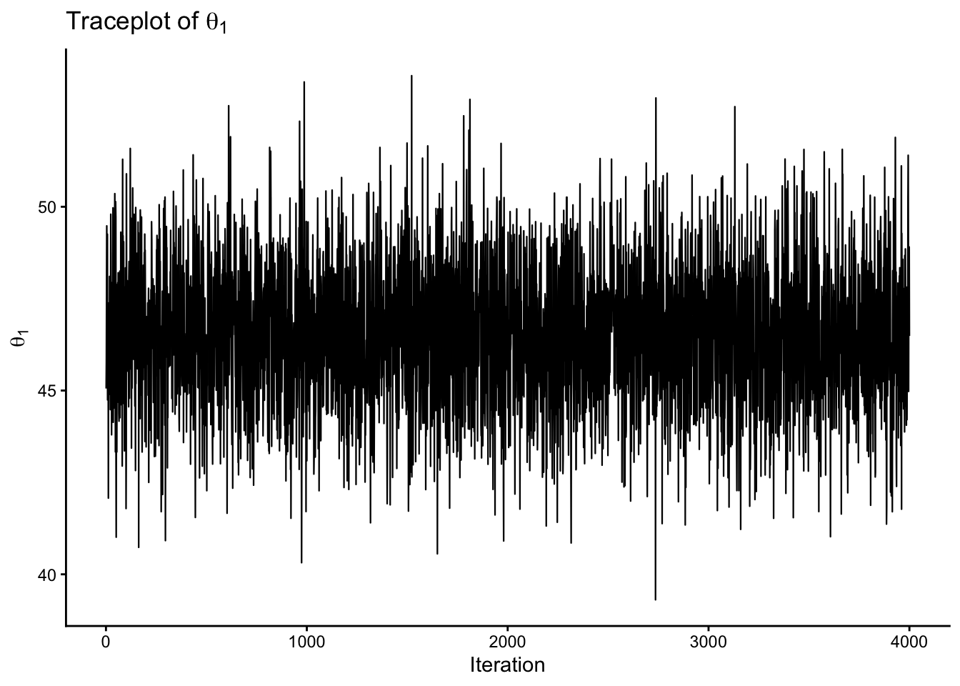
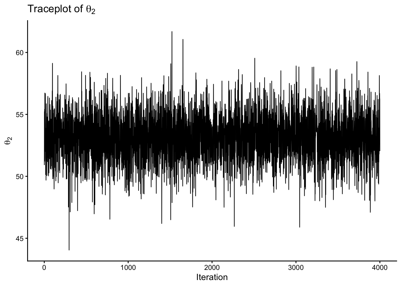
library(MASS)
library(ggplot2)

set.seed(8310)

# Simulated bivariate data
n <- 50
theta_true <- c(48, 54)
Sigma_true <- matrix(c(180, 95,
                       95, 240), 2, 2)

Y <- MASS::mvrnorm(n, mu = theta_true, Sigma = Sigma_true)
ybar <- colMeans(Y)

# Prior hyperparameters
mu0 <- c(50, 50)
Lambda0 <- matrix(c(625, 312.5,
                    312.5, 625), 2, 2)
nu0 <- 4
S0 <- Lambda0

# Storage
S <- 4000
THETA <- matrix(NA, nrow = S, ncol = 2)
SIGMA <- array(NA, dim = c(2, 2, S))

# Initial value
Sigma <- cov(Y)

for (s in 1:S) {
  # Update theta
  Lambda_n <- solve(solve(Lambda0) + n * solve(Sigma))
  mu_n <- Lambda_n %*% (solve(Lambda0) %*% mu0 + n * solve(Sigma) %*% ybar)
  theta <- as.numeric(MASS::mvrnorm(1, mu = mu_n, Sigma = Lambda_n))

  # Update Sigma
  S_theta <- matrix(0, 2, 2)
  for (i in 1:n) {
    d <- matrix(Y[i, ] - theta, ncol = 1)
    S_theta <- S_theta + d %*% t(d)
  }
  S_n <- S0 + S_theta
  Sigma <- solve(rWishart(1, df = nu0 + n, Sigma = solve(S_n))[,,1])

  THETA[s, ] <- theta
  SIGMA[, , s] <- Sigma
}

7.16.1 Traceplots for the posterior mean components

trace_df <- data.frame(
  iter = 1:S,
  theta1 = THETA[, 1],
  theta2 = THETA[, 2]
)

p1 <- ggplot(trace_df, aes(x = iter, y = theta1)) +
  geom_line(linewidth = 0.4) +
  labs(x = "Iteration", y = expression(theta[1]), title = expression("Traceplot of " * theta[1])) +
  theme_classic()

p2 <- ggplot(trace_df, aes(x = iter, y = theta2)) +
  geom_line(linewidth = 0.4) +
  labs(x = "Iteration", y = expression(theta[2]), title = expression("Traceplot of " * theta[2])) +
  theme_classic()

p1
p2

Figure 7.4: Traceplots of the two components of the posterior mean vector from a Gibbs sampler.

Figure 7.5: Traceplots of the two components of the posterior mean vector from a Gibbs sampler.

7.17 Missing data and imputation

A major application of the multivariate Gaussian model is missing-data imputation.

Suppose some components of \(\mathbf{Y}_i\) are missing. If the data are missing at random, then the observed part of each vector still contributes information about the mean and covariance, and the missing part can be sampled from its conditional distribution given the observed part.

This is attractive because:

we do not discard incomplete observations,
we account for uncertainty about the missing values,
we preserve dependence among variables.

Hoff emphasises that this is much better than either:

deleting incomplete cases, or
plugging in fixed values such as column means.

Important Bayesian lesson

Missing data can often be treated as additional unknown quantities rather than nuisances to be discarded.

7.18 Why this chapter matters for the rest of the course

This chapter is a bridge between basic Bayesian models and more sophisticated Bayesian workflows.

Once we can work with multivariate Gaussian distributions, we can move naturally to

hierarchical normal models,
Bayesian regression,
mixed-effects models,
latent Gaussian models,
Gaussian copulas and Gaussian processes.

So this chapter is foundational not only for multivariate data analysis, but for much of modern Bayesian modelling.

7.19 Summary

The multivariate Gaussian distribution is one of the cornerstones of Bayesian statistics.

Main ideas:

the mean vector controls location,
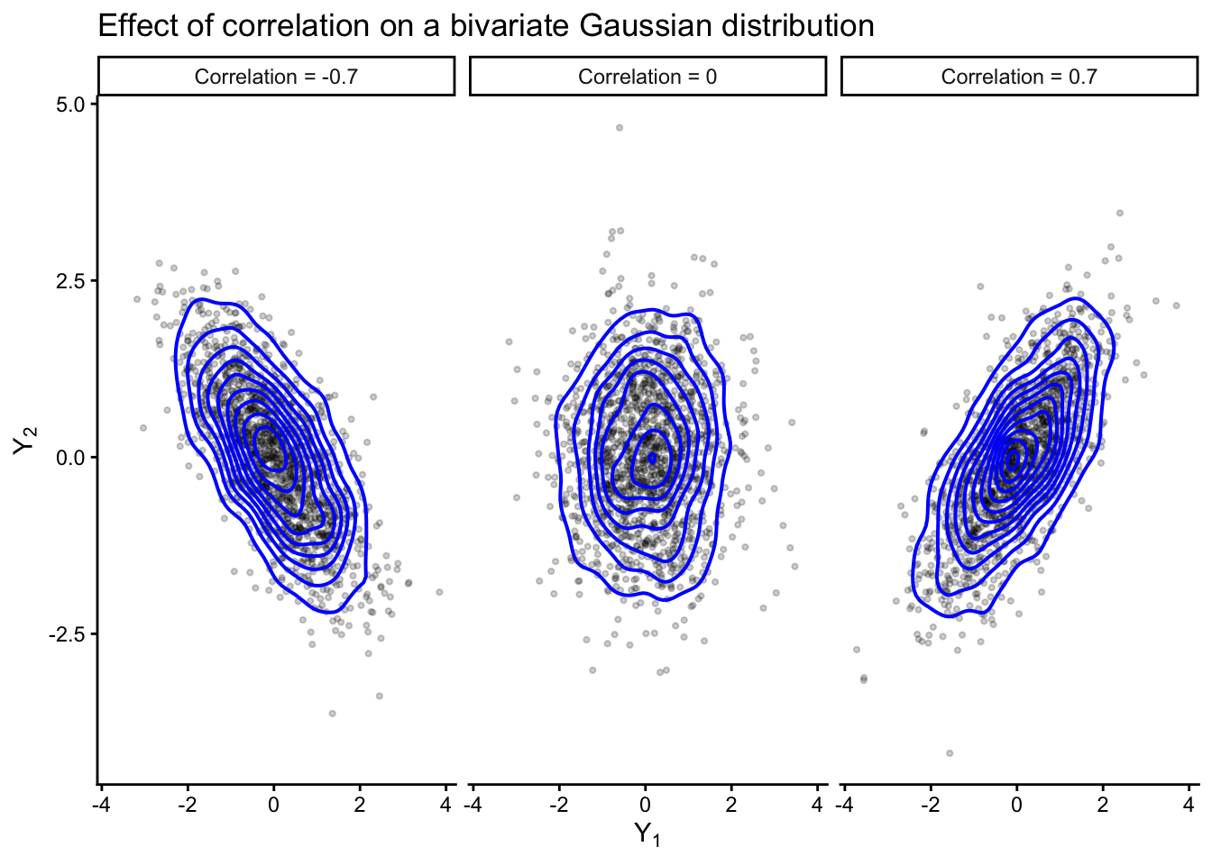
the covariance matrix controls spread and dependence,
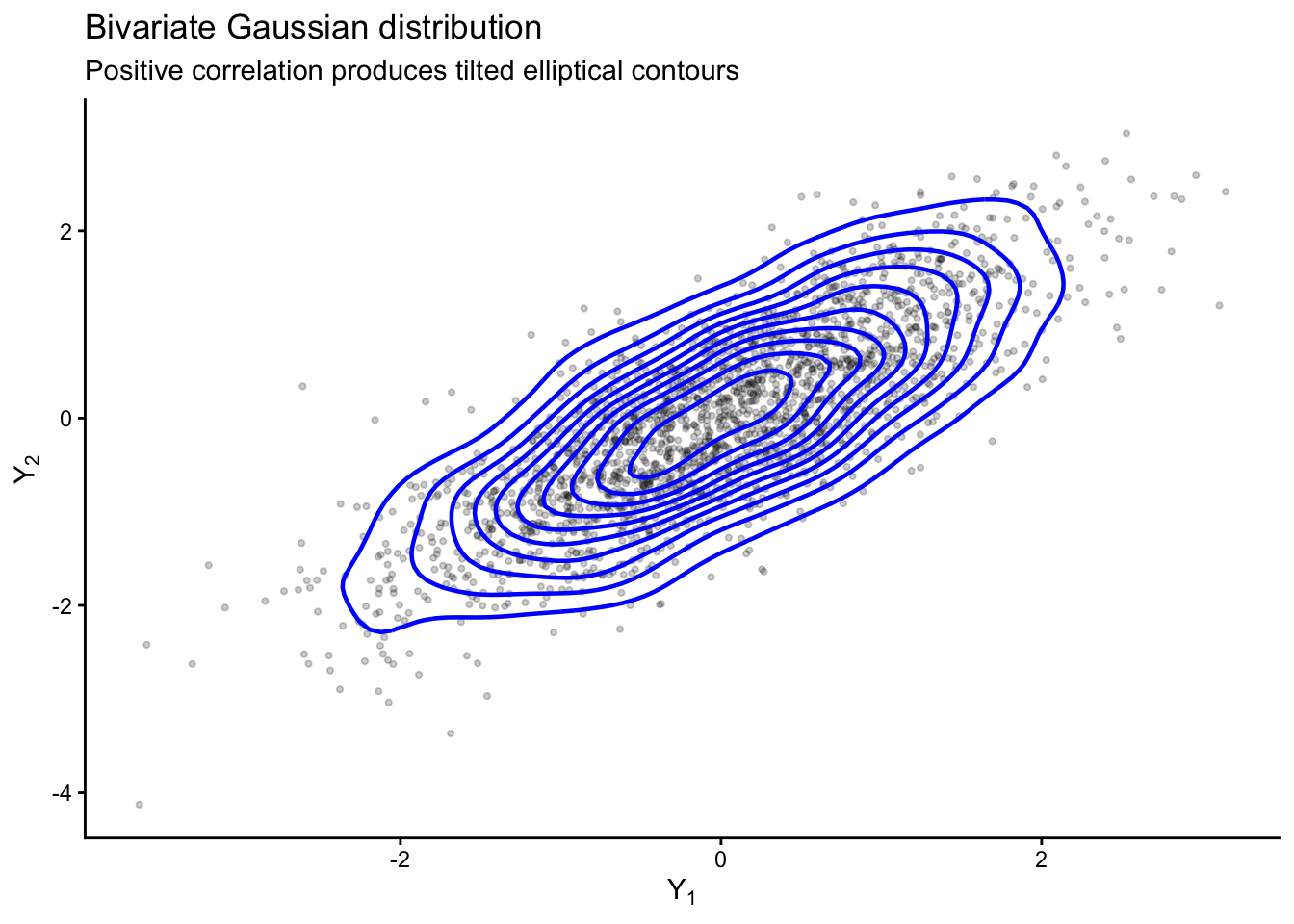
the geometry is elliptical,
marginal distributions are Gaussian,
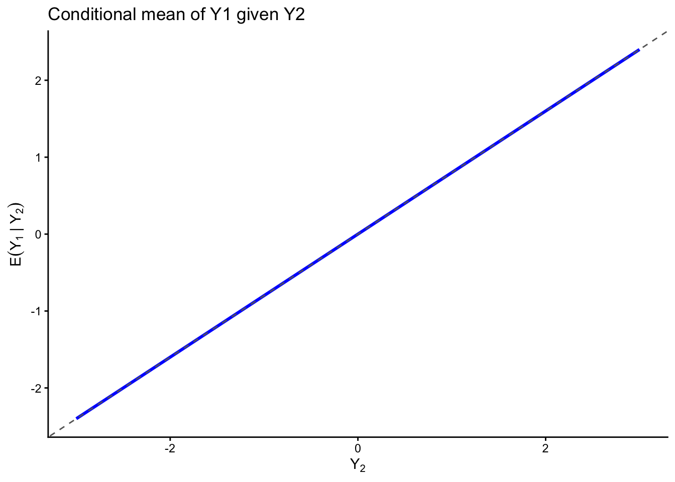
conditional distributions are Gaussian,
convenient priors lead to tractable full conditional distributions,
Gibbs sampling becomes feasible,
missing data can be imputed naturally.

In short,

\[ \begin{aligned} &\text{Multivariate Gaussian model} \\ &\;\Longrightarrow\; \text{joint modelling} \;+\; \text{tractable Bayesian computation}. \end{aligned} \]

7.20 Looking ahead

In the next parts of the chapter, we will continue to use this model to study:

semiconjugate priors for the mean vector,
inverse-Wishart priors for the covariance matrix,
Gibbs sampling of \((\boldsymbol{\theta},\boldsymbol{\Sigma})\),
and missing-data imputation.

This Chapter borrows materials from Chapter 7 in Hoff (2009).