8  Bayesian methods in Machine Learning: Regularization, Prediction, and Uncertainty

In this lecture, we explore several ways in which Bayesian statistics connects naturally with machine learning. The main message is that many ideas in modern machine learning have very natural Bayesian interpretations.

In particular, we will focus on three themes:

• regularization as prior modelling,
• prediction with uncertainty,
• Bayesian thinking in modern machine learning.

8.1 Why connect Bayesian statistics and machine learning?

Many machine learning methods are designed to do one or more of the following:

• estimate complicated models,
• make predictions,
• avoid overfitting,
• quantify uncertainty.

Bayesian methods are also designed to address these goals, but from a probabilistic perspective.

A Bayesian analysis starts with a model for the data, specifies prior distributions on unknown parameters, and then uses the posterior distribution to update beliefs and make predictions.

Note

A useful way to think about the connection is:

• machine learning often emphasizes prediction and optimization;
• Bayesian statistics emphasizes probability models and uncertainty quantification.

In many cases, the two perspectives are closely related.

8.2 Roadmap

In this lecture we will study:

1. Bayesian linear regression as a probabilistic prediction model,
2. regularization as prior modeling,
3. posterior predictive uncertainty,
4. why these ideas matter in modern machine learning.

8.3 Bayesian linear regression as probabilistic machine learning

Suppose we observe data

\[ (y_1,\mathbf{x}_1),\dots,(y_n,\mathbf{x}_n), \]

where each \(\mathbf{x}_i \in \mathbb{R}^p\) is a vector of predictors.

A standard linear regression model is

\[ y_i = \mathbf{x}_i^\top \boldsymbol{\beta} + \varepsilon_i, \qquad \varepsilon_i \sim \mathcal{N}(0,\sigma^2). \]

Equivalently,

\[ y_i \mid \boldsymbol{\beta},\sigma^2 \sim \mathcal{N}(\mathbf{x}_i^\top \boldsymbol{\beta},\sigma^2). \]

In matrix form,

\[ \mathbf{y} \mid \boldsymbol{\beta},\sigma^2 \sim \mathcal{N}_n(\mathbf{X}\boldsymbol{\beta}, \sigma^2 \mathbf{I}_n). \]

8.3.1 Frequentist view versus Bayesian view

In ordinary least squares regression, we estimate \(\boldsymbol{\beta}\) by a single point estimate:

\[ \hat{\boldsymbol{\beta}} = (\mathbf{X}^\top \mathbf{X})^{-1}\mathbf{X}^\top \mathbf{y}. \]

This gives one “best” coefficient vector.

In Bayesian linear regression, we instead treat \(\boldsymbol{\beta}\) as unknown and assign it a prior distribution, such as

\[ \boldsymbol{\beta} \sim \mathcal{N}_p(\mathbf{0}, \tau^2 \mathbf{I}_p). \]

Then we obtain the posterior distribution

\[ p(\boldsymbol{\beta} \mid \mathbf{y}, \mathbf{X}). \]

So instead of a single estimate, we get a full distribution over plausible values of the regression coefficients.

Note

This is one of the key Bayesian ideas in machine learning:

Instead of learning one parameter value, we learn a distribution over parameter values.

8.3.2 Why is this useful?

A posterior distribution over \(\boldsymbol{\beta}\) gives us:

• point estimates such as posterior means,
• interval estimates such as credible intervals,
• predictive distributions for new observations,
• uncertainty quantification.

This is especially useful when:

• sample sizes are small,
• predictors are correlated,
• overfitting is a concern,
• prediction uncertainty matters.

8.4 Regularization as prior modeling

One of the most important connections between Bayesian statistics and machine learning is that regularization can often be interpreted as a prior distribution.

8.4.1 Why regularization?

In machine learning, flexible models can easily overfit the data. To control complexity, we often add a penalty term.

For example, ridge regression solves

\[ \hat{\boldsymbol{\beta}}_{\text{ridge}} = \arg\min_{\boldsymbol{\beta}} \left\{ \sum_{i=1}^n (y_i - \mathbf{x}_i^\top \boldsymbol{\beta})^2 + \lambda \sum_{j=1}^p \beta_j^2 \right\}. \]

The second term penalizes large coefficients.

8.4.2 Bayesian interpretation of ridge regression

Suppose we use the Gaussian prior

\[ \beta_j \sim \mathcal{N}(0,\tau^2), \qquad j=1,\dots,p, \]

independently.

Then the log prior density is proportional to

\[ -\frac{1}{2\tau^2}\sum_{j=1}^p \beta_j^2. \]

Under a Gaussian likelihood, the log posterior is proportional to

\[ -\frac{1}{2\sigma^2}\sum_{i=1}^n (y_i - \mathbf{x}_i^\top \boldsymbol{\beta})^2 - \frac{1}{2\tau^2}\sum_{j=1}^p \beta_j^2. \]

Maximizing the posterior is therefore equivalent to minimizing a penalized least squares criterion. In particular, the Gaussian prior corresponds to an \(L_2\) penalty.

Important

A Gaussian prior on coefficients corresponds to ridge-type shrinkage.

So a prior is not only a statement about beliefs. It is also a way to control model complexity.

8.4.3 Bayesian interpretation of the lasso

The lasso solves

\[ \hat{\boldsymbol{\beta}}_{\text{lasso}} = \arg\min_{\boldsymbol{\beta}} \left\{ \sum_{i=1}^n (y_i - \mathbf{x}_i^\top \boldsymbol{\beta})^2 + \lambda \sum_{j=1}^p |\beta_j| \right\}. \]

This corresponds to a Laplace prior,

\[ p(\beta_j) \propto \exp(-\lambda |\beta_j|). \]

So:

• Gaussian prior \(\Rightarrow\) ridge-type shrinkage,
• Laplace prior \(\Rightarrow\) lasso-type shrinkage.

This is a powerful connection, because it shows that many machine learning penalties can be understood as prior distributions.

8.4.4 Why shrinkage is Bayesianly natural

From a Bayesian point of view, shrinkage happens because the prior says that very large coefficients are unlikely. The posterior combines this prior information with the evidence in the data.

This often improves prediction, especially in noisy or high-dimensional settings.

Note

In machine learning language: regularization controls overfitting.

In Bayesian language: priors regularize estimation.

8.5 A simple simulation: ordinary least squares versus ridge-style shrinkage

The following example illustrates the effect of shrinkage in a small regression problem.

library(ggplot2)

set.seed(8310)

n <- 40
p <- 8

X <- matrix(rnorm(n * p), nrow = n, ncol = p)
beta_true <- c(2, -1.5, 1, 0, 0, 0, 0, 0)
y <- X %*% beta_true + rnorm(n, sd = 2)
y <- as.numeric(y)

# OLS estimate
beta_ols <- solve(t(X) %*% X, t(X) %*% y)

# Ridge estimate
lambda <- 10
beta_ridge <- solve(t(X) %*% X + lambda * diag(p), t(X) %*% y)

coef_df <- data.frame(
  index = factor(1:p),
  True = beta_true,
  OLS = as.numeric(beta_ols),
  Ridge = as.numeric(beta_ridge)
)

coef_long <- rbind(
  data.frame(index = coef_df$index, value = coef_df$True, method = "True"),
  data.frame(index = coef_df$index, value = coef_df$OLS, method = "OLS"),
  data.frame(index = coef_df$index, value = coef_df$Ridge, method = "Ridge")
)

ggplot(coef_long, aes(x = index, y = value, fill = method)) +
  geom_col(position = "dodge") +
  labs(
    title = "OLS and ridge estimates",
    x = "Coefficient index",
    y = "Value",
    fill = NULL
  ) +
  theme_classic()

Figure 8.1: Comparison of ordinary least squares and ridge regression coefficient estimates in a small simulated example.

8.6 Discussion of the plot

In many small or noisy datasets, the ordinary least squares estimates can be unstable. Ridge shrinkage tends to pull the estimates toward zero. This can reduce variance and improve predictive performance, even if it introduces some bias.

This is a good example of a more general machine learning principle:

A small amount of bias can be worthwhile if it substantially reduces variance.

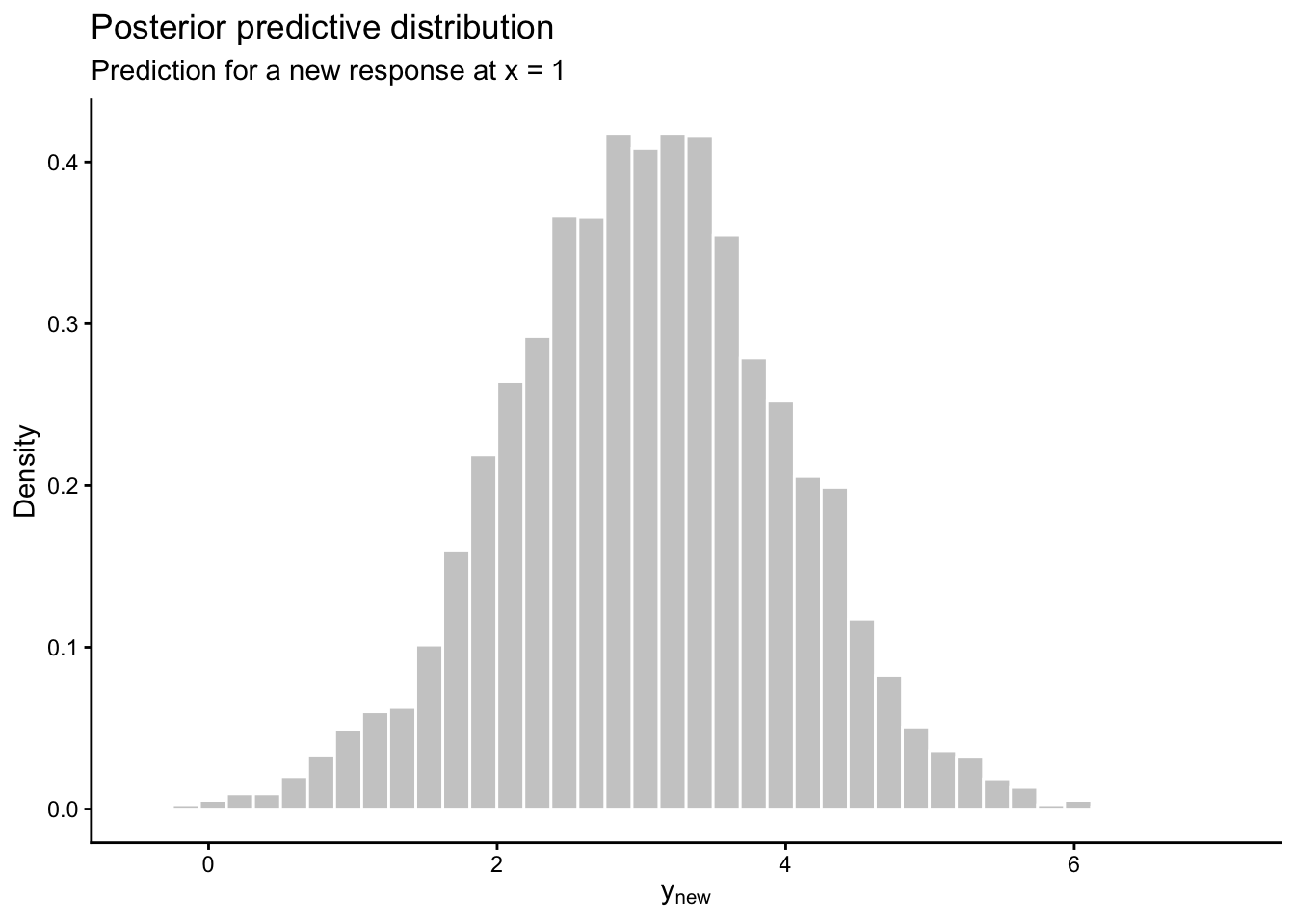
8.7 Prediction and uncertainty

A major strength of Bayesian methods is that prediction is naturally probabilistic.

Suppose we have a new predictor vector \(\mathbf{x}_{\text{new}}\). In a non-Bayesian regression analysis, we may plug in an estimate and compute

\[ \hat{y}_{\text{new}} = \mathbf{x}_{\text{new}}^\top \hat{\boldsymbol{\beta}}. \]

In a Bayesian analysis, we instead use the posterior predictive distribution

\[ p(y_{\text{new}} \mid \mathbf{y}) = \int p(y_{\text{new}} \mid \boldsymbol{\beta},\sigma^2)\, p(\boldsymbol{\beta},\sigma^2 \mid \mathbf{y})\, d\boldsymbol{\beta}\,d\sigma^2. \]

This distribution accounts for both:

• randomness in future observations,
• uncertainty about the parameters.

8.8 Why posterior predictive distributions matter

Posterior predictive distributions are useful because they let us answer questions such as:

• What values are plausible for a future outcome?
• How uncertain is our prediction?
• How do different models compare in predictive performance?

This is especially important in decision-making problems, where uncertainty is not a nuisance but a core part of the problem.

Important

Machine learning models often emphasize accurate prediction.

Bayesian models emphasize accurate prediction with calibrated uncertainty.

8.9 A simple predictive simulation

The next example illustrates posterior predictive thinking in a regression setting. For simplicity, we simulate from a Gaussian approximation.

library(MASS)
library(ggplot2)

set.seed(8310)

n <- 50
x <- runif(n, -2, 2)
y <- 1 + 2 * x + rnorm(n, sd = 1)

X <- cbind(1, x)
beta_hat <- solve(t(X) %*% X, t(X) %*% y)
sigma2_hat <- sum((y - X %*% beta_hat)^2) / (n - 2)
V_beta <- sigma2_hat * solve(t(X) %*% X)

# Simulate approximate posterior draws
S <- 4000
beta_draws <- MASS::mvrnorm(S, mu = as.numeric(beta_hat), Sigma = V_beta)

x_new <- 1.0
X_new <- c(1, x_new)

y_new_draws <- numeric(S)
for (s in 1:S) {
  mu_new <- sum(X_new * beta_draws[s, ])
  y_new_draws[s] <- rnorm(1, mean = mu_new, sd = sqrt(sigma2_hat))
}

pred_df <- data.frame(y_new = y_new_draws)

ggplot(pred_df, aes(x = y_new)) +
  geom_histogram(aes(y = after_stat(density)),
                 bins = 40,
                 fill = "grey80",
                 color = "white") +
  labs(
    title = "Posterior predictive distribution",
    subtitle = "Prediction for a new response at x = 1",
    x = expression(y[new]),
    y = "Density"
  ) +
  theme_classic()

Figure 8.2: Posterior predictive distribution for a new observation in a simple regression example.

8.10 What do we learn from this?

This histogram is not just a point prediction. It is a distribution for the future observation.

From it, we can compute:

• predictive means,
• predictive intervals,
• probabilities of exceeding a threshold.

This is often much more useful than a single fitted value.

8.11 Bayesian ideas in modern machine learning

The ideas we have seen so far are not isolated topics. They reappear in many modern machine learning methods.

8.11.1 1. Priors as regularizers

We have already seen that priors can act like penalties. This idea extends far beyond ridge and lasso.

Examples:

• Gaussian priors \(\Rightarrow\) shrinkage,
• Laplace priors \(\Rightarrow\) sparsity,
• hierarchical priors \(\Rightarrow\) adaptive shrinkage.

8.11.2 2. Prediction with uncertainty

Many machine learning models make predictions, but not all provide uncertainty in a principled way.

Bayesian models naturally provide:

• predictive distributions,
• credible intervals,
• probabilities of events.

This is particularly important in applications such as:

• medicine,
• policy,
• finance,
• scientific prediction.

8.11.3 3. Model complexity and overfitting

Bayesian methods can control complexity through the prior. Instead of just asking

Which parameter values fit the data best?

Bayesian analysis asks

Which parameter values are plausible after combining prior structure with the observed data?

This can improve stability and generalization.

8.11.4 4. Modern computation

In simple models, posterior distributions may be available in closed form. In more complicated models, Bayesian machine learning relies on computational methods such as:

• MCMC,
• Hamiltonian Monte Carlo,
• variational inference.

This is one reason Bayesian computation has become such an important part of modern statistics and machine learning.

8.12 Bayesian versus machine learning language

It is often helpful to translate between the two languages.

Machine learning language	Bayesian language
Regularization	Prior distribution
Training loss + penalty	Negative log posterior
Prediction	Posterior predictive distribution
Parameter estimate	Posterior summary
Ensemble / uncertainty	Posterior distribution over functions or parameters

Note

These are not exactly the same in every setting, but the parallels are often very strong.

8.13 What Bayesian methods add

It is worth emphasizing that Bayesian methods do not replace machine learning. Rather, they provide a probabilistic framework for many of the same goals.

Bayesian methods add:

• principled uncertainty quantification,
• coherent updating,
• interpretable regularization through priors,
• predictive distributions instead of only point predictions.

8.14 Summary

In this lecture, we explored several important links between Bayesian statistics and machine learning.

Main ideas:

• Bayesian linear regression is a probabilistic predictive model.
• Regularization can often be interpreted as prior modeling.
• Posterior predictive distributions quantify uncertainty in predictions.
• Many modern machine learning ideas have natural Bayesian counterparts.

In short,

\[ \text{Bayesian statistics} \;\Longleftrightarrow\; \text{probabilistic machine learning}. \]