9  Modern Bayesian Computation and Models

In the previous lecture, we discussed several connections between Bayesian statistics and machine learning (ML), focusing on

• Bayesian linear regression,
• regularization as prior modelling,
• and posterior predictive uncertainty.

In this lecture, we continue that theme by looking at two major directions in modern Bayesian statistics:

• modern Bayesian computation, especially variational inference;
• modern Bayesian modelling, especially Gaussian processes.

The main message of this lecture is:

Modern Bayesian statistics is not only about priors and posteriors. It is also about how to compute them efficiently and how to build flexible probabilistic models.

9.1 Roadmap

In this lecture we will study:

1. why classical MCMC is not always enough,
2. variational inference as optimization-based Bayesian approximation,
3. Gaussian processes as priors over functions,
4. why these ideas matter in modern statistics and ML

Question: Why do we need modern Bayesian computation?

So far in this course, we have focused heavily on models where posterior inference is tractable or can be handled using Gibbs sampling.

This works very well in many classical Bayesian models. However, in modern applications, we often encounter:

• high-dimensional parameter spaces,
• nonconjugate models,
• large datasets,
• complex posterior geometry.

In such situations, exact posterior sampling may be slow or difficult.

Note

The main computational challenge in Bayesian statistics is:

How do we approximate a posterior distribution accurately enough, but also efficiently enough, for modern problems?

9.2 A short review of MCMC

MCMC methods approximate posterior distributions by generating dependent samples

\[ \phi^{(1)},\dots,\phi^{(S)} \]

from a MC whose stationary distribution is the target posterior.

Then posterior expectations are approximated by

\[ E[g(\phi)\mid y] \approx \frac{1}{S}\sum_{s=1}^S g(\phi^{(s)}). \]

This is a powerful idea, but MCMC can become computationally expensive when:

• the chain mixes slowly,
• the dimension is large,
• the likelihood is costly to evaluate,
• or we need to analyze many datasets quickly.

9.3 Beyond classical MCMC

Modern Bayesian computation includes methods such as

• Hamiltonian MC,
• variational inference,
• stochastic gradient MCMC,
• approximate Bayesian computation.

In this lecture, we focus on variational inference, because it is one of the clearest examples of the connection between Bayesian computation and ML

9.4 Variational inference

9.4.1 Core idea

Suppose the true posterior is

\[ p(\theta \mid y), \]

but this distribution is hard to compute or sample from directly.

Instead of drawing MCMC samples, variational inference approximates the posterior by choosing a simpler distribution

\[ q(\theta) \]

from a family of tractable distributions, and then finding the member of that family \(\mathcal{Q}\) that is “closest” to the posterior.

The approximation problem becomes

\[ q^*(\theta) = \arg\min_{q \in \mathcal{Q}} \mathrm{KL}\bigl(q(\theta)\,\|\,p(\theta\mid y)\bigr). \]

So variational inference turns posterior approximation into an optimization problem.

Important

MCMC is based on sampling.

Variational inference is based on optimization.

Why is this useful?

Variational inference can be much faster than MCMC, especially in large or complicated models. This is one reason it is widely used in ML and large-scale Bayesian modelling.

The tradeoff is that the approximation may be biased, because we are restricting attention to a smaller family of distributions.

The Kullback–Leibler (KL) divergence from \(q\) to \(p\) is

\[ \mathrm{KL}(q \,\|\, p) = \int q(\theta)\log \frac{q(\theta)}{p(\theta\mid y)}\,d\theta. \]

This quantity is always nonnegative, and it equals zero only if \(q = p\) almost everywhere.

So minimizing KL divergence tries to make \(q\) as close as possible to the posterior.

9.4.2 The ELBO

Directly minimizing

\[ \mathrm{KL}(q(\theta)\,\|\,p(\theta\mid y)) \]

is not always convenient, because the posterior normalization constant may be unknown.

Instead, variational inference often maximizes the evidence lower bound (ELBO),

\[ \mathrm{ELBO}(q) = E_q[\log p(y,\theta)] - E_q[\log q(\theta)]. \]

Maximizing the ELBO is equivalent to minimizing the KL divergence.

Interpretation of the ELBO

The ELBO has two parts:

• a fit term, which encourages \(q\) to place mass where the joint density \(p(y,\theta)\) is large;
• an entropy term, which discourages \(q\) from collapsing too much.

This balance is similar in spirit to many machine learning optimization problems, where we balance fit and complexity.

9.4.3 Mean-field variational inference

A common simplification is to assume that the approximation factorizes:

\[ q(\theta) = \prod_{j=1}^p q_j(\theta_j). \]

This is called the mean-field approximation.

It makes optimization easier, but it can underestimate posterior dependence.

Warning

A common limitation of variational inference is that it may underestimate posterior uncertainty, especially when the true posterior has strong dependence.

9.4.4 Variational inference versus MCMC

The table below summarizes the broad comparison.

Feature	MCMC	Variational inference
Main idea	Sampling	Optimization
Accuracy	Often high	Approximate
Speed	Can be slow	Often faster
Output	Samples from posterior	Approximate distribution
Uncertainty quantification	Usually strong	May be underestimated

9.4.5 A simple variational approximation example

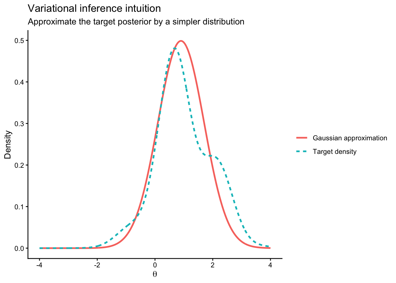
The following code illustrates a very simple variational-style approximation idea. We compare a target density with a Gaussian approximation.

This is not a full general-purpose VI algorithm. The goal is only to build intuition.

library(ggplot2)

theta_grid <- seq(-4, 4, length.out = 1000)

# Example target density: a non-Gaussian posterior-like shape
target_unnorm <- exp(-0.5 * (theta_grid - 1)^2) * (1 + 0.3 * sin(3 * theta_grid))
target_unnorm[target_unnorm < 0] <- 0
target_density <- target_unnorm / sum(target_unnorm) / (theta_grid[2] - theta_grid[1])

# A simple Gaussian approximation
q_density <- dnorm(theta_grid, mean = 0.9, sd = 0.8)

df_vi <- data.frame(
  theta = rep(theta_grid, 2),
  density = c(target_density, q_density),
  curve = factor(rep(c("Target density", "Gaussian approximation"),
                     each = length(theta_grid)))
)

ggplot(df_vi, aes(x = theta, y = density, color = curve, linetype = curve)) +
  geom_line(linewidth = 1) +
  labs(
    title = "Variational inference intuition",
    subtitle = "Approximate the target posterior by a simpler distribution",
    x = expression(theta),
    y = "Density",
    color = NULL,
    linetype = NULL
  ) +
  theme_classic()

Figure 9.1: A target density and a simple Gaussian approximation.

9.4.6 Takeaway from variational inference

Variational inference is attractive because it scales well and turns Bayesian inference into optimization. This makes it very natural for modern machine learning.

At the same time, we should remember:

• it is an approximation,
• its quality depends on the approximation family,
• and it may not capture all posterior dependence or uncertainty.

9.5 Gaussian processes

We now turn to a different modern Bayesian idea: Gaussian processes (GP).

Whereas variational inference is mainly about computation, GPs are mainly about modelling.

9.5.1 Motivation

In regression, we often assume a parametric relationship such as

\[ y_i = \beta_0 + \beta_1 x_i + \varepsilon_i. \]

But what if the true relationship is nonlinear and we do not want to commit to a specific parametric form?

A GP provides a Bayesian way to model an unknown function flexibly.

9.5.2 Core idea

In GP regression, we write

\[ y_i = f(x_i) + \varepsilon_i, \qquad \varepsilon_i \sim \mathcal{N}(0,\sigma^2), \]

and then place a prior directly on the unknown function \(f\).

A GP prior says that for any collection of inputs

\[ x_1,\dots,x_n, \]

the corresponding function values

\[ (f(x_1),\dots,f(x_n))^\top \]

follow a multivariate Gaussian distribution.

In symbols,

\[ f \sim \mathcal{GP}(m(\cdot), k(\cdot,\cdot)), \]

where

• \(m(x)\) is the mean function,
• \(k(x,x')\) is the covariance kernel.

Note

A GP is an infinite-dimensional generalization of the multivariate Gaussian distribution.

This is exactly why GP fit naturally after our earlier lecture on multivariate Gaussian models.

9.5.3 The kernel function

The kernel

\[ k(x,x') \]

determines how strongly the function values at \(x\) and \(x'\) are related.

A common choice is the squared exponential kernel:

\[ k(x,x') = \alpha^2 \exp\left( -\frac{(x-x')^2}{2\ell^2} \right), \]

where

• \(\alpha^2\) controls vertical variability,
• \(\ell\) controls smoothness.

Large \(\ell\) leads to smoother functions. Small \(\ell\) allows more rapid local variation.

9.5.4 Why Gaussian processes are Bayesian

GP regression is Bayesian because:

• we specify a prior over functions,
• data update this prior to a posterior over functions,
• prediction is based on the posterior predictive distribution.

So the output is not just one estimated curve. It is a posterior distribution over plausible curves.

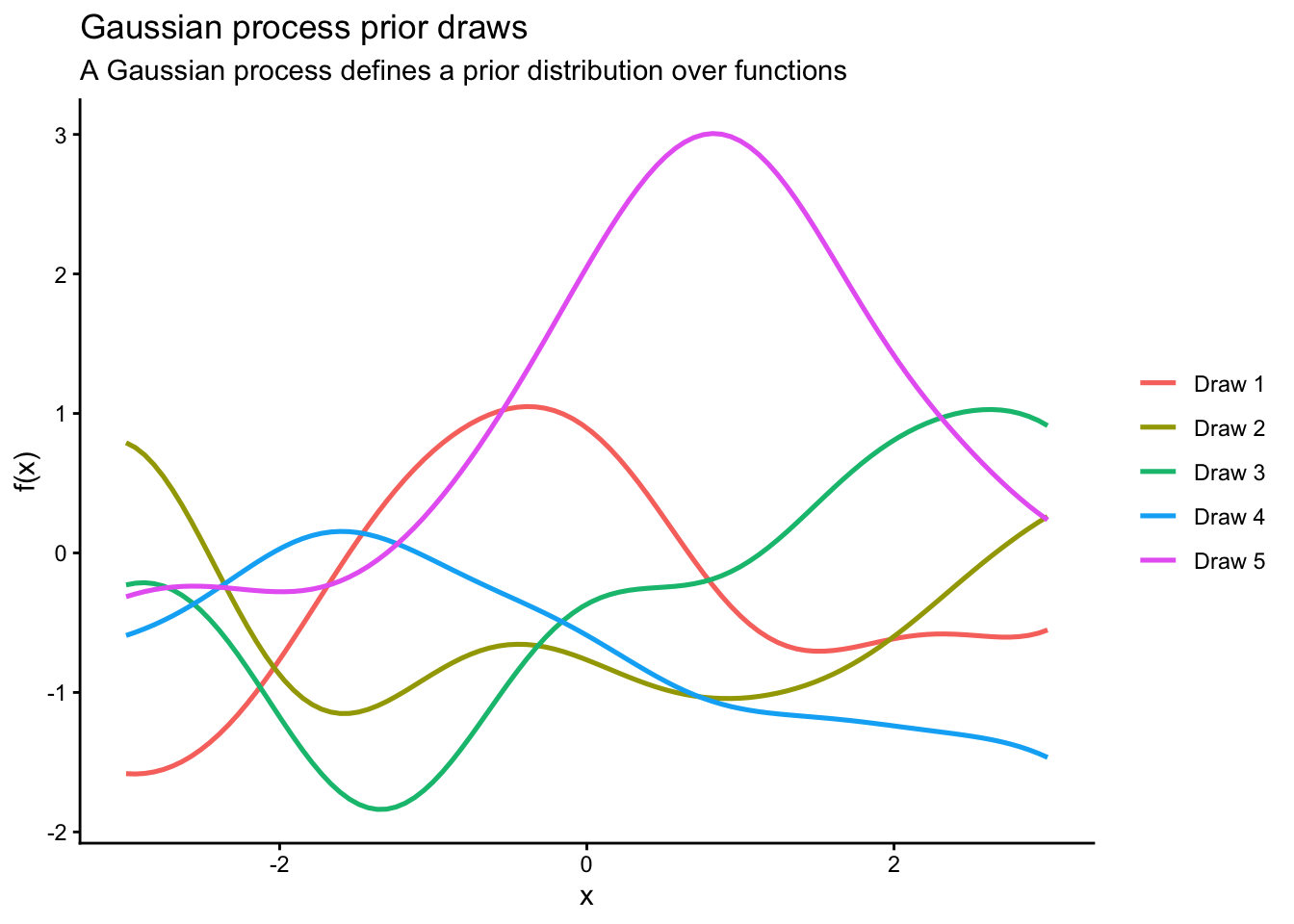
9.5.5 Simulating prior draws from a GP

The following example illustrates the idea of a prior over functions.

library(MASS)
library(ggplot2)

set.seed(8310)

x_grid <- seq(-3, 3, length.out = 100)

kernel_se <- function(x1, x2, alpha = 1, ell = 1) {
  alpha^2 * exp(-(outer(x1, x2, "-")^2) / (2 * ell^2))
}

K <- kernel_se(x_grid, x_grid, alpha = 1, ell = 1)
K <- K + 1e-8 * diag(length(x_grid))  # numerical stability

gp_draws <- MASS::mvrnorm(5, mu = rep(0, length(x_grid)), Sigma = K)

gp_df <- do.call(rbind, lapply(1:5, function(j) {
  data.frame(x = x_grid, y = gp_draws[j, ], draw = factor(paste("Draw", j)))
}))

ggplot(gp_df, aes(x = x, y = y, color = draw)) +
  geom_line(linewidth = 0.9) +
  labs(
    title = "Gaussian process prior draws",
    subtitle = "A Gaussian process defines a prior distribution over functions",
    x = "x",
    y = "f(x)",
    color = NULL
  ) +
  theme_classic()

Figure 9.2: Draws from a Gaussian process prior.

9.5.6 Why Gaussian processes matter

GPs are important because they combine:

• flexible nonlinear regression,
• uncertainty quantification,
• elegant Bayesian updating.

They are widely used in:

• spatial statistics,
• Bayesian optimization,
• surrogate modeling,
• computer experiments,
• probabilistic machine learning.

9.5.7 GPs and multivariate Gaussian distributions

A Gaussian process is built from multivariate Gaussian distributions. If we evaluate the unknown function at finitely many input points, then the resulting vector is multivariate Gaussian.

So the structure is:

\[ f \sim \mathcal{GP}(m,k) \quad \Longrightarrow \quad (f(x_1),\dots,f(x_n))^\top \sim \mathcal{N}_n(\mathbf{m}, \mathbf{K}). \]

This is one reason the multivariate Gaussian distribution is so central in modern Bayesian modeling.

9.6 Bigger picture: modern Bayesian statistics

We can now summarize two big themes.

Theme 1: Bayesian computation

Modern Bayesian methods often need computational tools beyond closed-form conjugate analysis.

Examples include:

• MCMC,
• Hamiltonian Monte Carlo,
• variational inference.

Theme 2: Bayesian modeling

Modern Bayesian statistics also provides very flexible modeling tools.

Examples include:

• hierarchical models,
• Gaussian processes,
• latent variable models,
• Bayesian neural networks.

These ideas allow us to model uncertainty in complicated problems while still keeping a probabilistic interpretation.

9.6.1 Bayesian and machine learning: a broader view

At this point, we can see that Bayesian statistics and machine learning overlap in several deep ways.

Machine learning perspective	Bayesian perspective
Optimization	Posterior approximation
Regularization	Prior modeling
Flexible function fitting	Nonparametric Bayes / Gaussian processes
Predictive modeling	Posterior predictive inference
Ensemble uncertainty	Distribution over parameters or functions

Note

Bayesian statistics does not replace ML Rather, it provides a principled probabilistic framework for many ML goals.

NoneTake home message

If you remember only a few things from this lecture, they should be:

1. Modern Bayesian inference often requires approximation.
   Variational inference is one major example.

2. Modern Bayesian models can be highly flexible.
   Gaussian processes are one major example.

3. Bayesian methods provide more than point estimates.
   They provide uncertainty quantification for parameters, functions, and predictions.

9.7 Summary

In this lecture, we studied two important modern Bayesian ideas.

Variational inference

• turns posterior approximation into optimization,
• is often faster than MCMC,
• but may introduce approximation bias.

Gaussian processes

• define priors over functions,
• extend multivariate Gaussian ideas to infinite-dimensional settings,
• provide flexible nonlinear regression with uncertainty quantification.

In short,

\[ \text{Modern Bayesian statistics} \;=\; \text{probabilistic modeling} \;+\; \text{modern computation}. \]

9.8 Looking back on the course

This course has moved from:

• basic Bayesian probability and prior-posterior updating,
• conjugate models,
• MC approximation,
• Gibbs sampling and diagnostics,
• multivariate Gaussian models,

to ideas that connect directly to modern ML and modern Bayesian data analysis.

The underlying message has stayed the same:

Bayesian statistics is a coherent way to model uncertainty, learn from data, and make predictions.